2019年第八届数学建模国际赛小美赛B题数据中心冷出风口的设计解题全过程文档及程序
2019年第八届数学建模国际赛小美赛
B题 数据中心冷出风口的设计
原题再现:
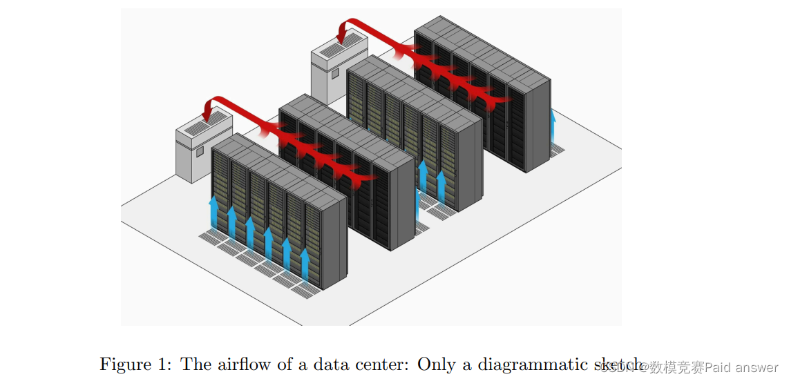
??这是数据中心空调设计面临的一个问题。在一些数据中心,计算机机柜是开放的,在一个房间里排列成三到四排。冷却后的空气通过主管进入房间,并分为三到四个支管。支管的出口只能放在天花板上,向下吹,热空气从房间一侧的热空气安全壳中排出。每个支管的出口不应超过三个1。由于冷空气和热空气的混合,冷空气的利用效率降低。因此,我们需要考虑空气流量,以减少走廊和缝隙中浪费的制冷量。
??我们需要考虑天花板的高度、橱柜的高度以及不同橱柜的典型热输出。我们假设空调的总制冷量能够满足机房的运行要求。当我们确定机柜的布局时,如何设置空调出风口的位置是最好的解决方案?
整体求解过程概述(摘要)
??数据通信机房是一个巨大的耗能系统。近年来,随着网络通信技术的飞速发展,在机房的建设和改造过程中,面临着许多能源和安全问题。为了保证数据通信机房的高效冷却和安全运行的重要保证,运营商希望在正常工作的前提下改善机房内的气流组织,并在消除可能的安全隐患的前提下,将散热、功耗降至最低。针对此类工程应用问题,本文对机房空调配置及运行状况进行了综合评价。基于ANSYS的icepak模块,成功构建了机房内部温度场和气流方向,建立了机房数学模型,模拟了机房温度场。对数据通信机房的分布状况、冷负荷核算、实验设计和优化进行了研究。最后,建立筛选软件,提供不同的冷却方案。
??首先分析了机房的俯视图、侧视图和主视图,并在每个视图中设置了敏感区域和路径的特殊点。由于机房内的温度随时间呈线性变化,但随位置变化具有明显的区域性特征,为了能够简单地获得温度情况,可以对机房内的温度变化进行有限元模拟,在仿真结果中可以方便地得到特殊点的温度。在设定的路径上进行曲线拟合,得到温度随位置变化的函数。由于计算机室内的空间是特定的,通过在所有空间中依次设置路径,可以很容易地检测到空间中的任何位置的温度变化。然后对温度进行时间积分,得到热的变化。
模型假设:
??1、各种材料的导热系数是恒定的,不随时间变化。
??2、各出风口风量始终相同。
??3、各风口风速为固定值。
??4、假设不存在能源浪费(冷水机组效率为100%),达到机房设定温度所需的冷量为合理的参考冷负荷。
??5、假设日常空调运行前机房内外温度相同。
??6、假设机房电气设备冷负荷全年不变。
??7、假设房间位置的温度是恒定的。
??8、忽略空调内部水管阻力和自身能耗。
??9、假设出风口位置、底盘高度、室内吊顶高度、底盘类型为自变量。
??10、假设底盘随高度增加,热量均匀增加。
问题分析:
??由于支管的位置只能放在顶棚上,风冷气体只能从顶棚吹出,在顶棚处可以改变冷却气体的出口位置,以达到最佳的冷却效果。对于不同类型的出风口位置,可设置不同类型的机柜放电。由于从天花板吹来的冷却气体密度较高,部分气体与走廊和缝隙中的热风混合,消耗不必要的冷却,不会显著降低机柜的热量。这部分气体理论上需要实现。增加冷却效率的最小值。
??由于机柜的高度将直接影响机柜中服务器的数量,从而影响总产热量,因此机柜的高度对提高冷却效率起着重要作用。由于重力的下降,从天花板上的冷却气体出口吹出的冷却气体在不同高度会产生不同的影响。在最高空气温度下,冷却气体的密度高于冷却气体的密度,且冷却气体的下降速度较快。在逐渐下降的过程中,由于机柜释放的热量的影响,一些较热的气体和冷却气体混合,使冷却气体的温度逐渐上升和下降。冷却气体吸收并混合底盘在干燥垂直方向释放的所有热量,由于冷却气体的温升和温降速率,这部分气体的温度达到最大值。升温气体继续上升,为保证带走底盘热量的冷却气体能及时排出室外,冷却气体出口应尽量远离出口风口,以便及时带走底盘热量,但此时,离冷却口最远的机柜会因为少量冷却而达到非常高的温度。另外,由于不同的散热方式和不同机柜的散热方式不同,周围空气的热传导也不同,因此不同类型的机柜对散热也有重要影响。
??为了说明这一问题,本文设置了两组实验。第一组实验在风口在吊顶上位置固定的情况下,确定影响室内总冷量的主要因素,并采用显著性检验确定影响室内总冷量的主要因素。通过检验,计算显著性系数,粗略确定影响因素权重,建立底盘高度、室内吊顶高度与底盘类型之间的函数关系。第二组测试在确定箱体高度、室内天花板高度和底盘类型之间作为变量的函数关系的基础上,重置天花板上出风口的位置。
模型的建立与求解整体论文缩略图
全部论文请见下方“ 只会建模 QQ名片” 点击QQ名片即可
部分程序代码:(代码和文档not free)
function main()
clc % clear screen
clear all; % clear memory armor to speed up computing
close all; % current figure images
warning off; % mask does not have the necessary warning
SamNum=20; % input sample number is 20
TestSamNum=20; % test sample size is 20
ForcastSamNum=2;% predicted sample size is 2
HiddenUnitNum=8;% in the middle layer the number of hidden layers is 8
InDim=3; % network input dimension is 3
OutDim=2; % network output size is 2

% Raw data
%
sqrs=[0.46 0.46 0.46 0.44 0.44 0.44
0.35 0.50 0.50 0.48 0.48 0.47
0.30 0.55 0.52 0.45 0.50 0.45
0.23 0.59 0.55 0.46 0.53 0.40];
%
sqjdcs=[0.520.52 0.48 0.48 0.48
0.56 0.55 0.49 0.55 0.54
0.59 0.59 0.58 0.58 0.55
0.61 0.65 0.61 0.59 0.59
0.63 0.68 0.62 0.62 0.62];
sqglmj=[0.52 0.52 0.48 0.48 0.48
0.56 0.55 0.49 0.55 0.54
0.59 0.59 0.58 0.58 0.55
0.61 0.65 0.61 0.59 0.59
0.63 0.68 0.62 0.62 0.62];
%
glkyl=[0.52 0.52 0.48 0.48 0.48
0.56 0.55 0.49 0.55 0.54
0.59 0.59 0.58 0.58 0.55
0.61 0.65 0.61 0.59 0.59
0.63 0.68 0.62 0.62 0.62];
%
glhyl=[0.45 0.45 0.45 0.55 0.55 0.55
0.42 0.50 0.55 0.56 0.59 0.58
0.40 0.52 0.58 0.61 0.62 0.62
0.38 0.54 0.61 0.60 0.64 0.61
0.35 0.59 0.64 0.61 0.65 0.63];

p=[sqrs;sqjdcs;sqglmj]; % input data matrixt
t=[glkyl;glhyl]; % target data matrix
[SamIn,minp,maxp,tn,mint,maxt]=premnmx(p,t); % Initial sample pair (input and output) initialization

rand('state',sum(100*clock)); % Generate random numbers based on system clock seeds
NoiseVar=0.01; % noise intensity is 0.01 (the purpose of adding noise is to prevent network overfitting)
Noise=NoiseVar*randn(2,SamNum); % Generate noise
SamOut=tn+Noise; % Add noise to the output sample

TestSamIn=SamIn; % The input sample is the same as the test sample because the sample size is too small
TestSanOut=SamOut; % The output sample is the same as the test sample

MaxEpochs=50000; % Maximum training times is 50000
lr=0.035; % Learning rate is 0.035
E0=0.65*10^(-3); % Target error is 0.65*10^(-3)
W1=0.5*rand(HiddenUnitNum,InDim)-0.1;% Initializes the weight between the input layer and the hidden layer
B1=0.5*rand(HiddenUnitNum,1)-0.1;% Initializes the weight between the input layer and the hidden layer
W2=0.5*rand(OutDim,HiddenUnitNum)-0.1;% Initializes the weight between the output layer and the hidden layer
B2=0.5*rand(OutDim,1)-0.1;% Initialize the weight between the output layer and the hidden layer
ErrHistory=[]; % Pre-occupies memory for intermediate variables
for i=1:MaxEpochs
 HiddenOut=logsig(W1*SamIn+repmat(B1,1,SamNum)); % Hidden layer network output
 NetworkOut=W2*HiddenOut+repmat(B2,1,SamNum); % Output layer network output
 Error=SamOut-NetworkOut; % The difference between the actual output and the network output
 SSE=sumsqr(Error); % Energy function (square of error)
 ErrHistory=[ErrHistory SSE];
 if SSE<E0,break,end % Jump out of the learning loop if the error is met

 % The following 6 lines are the core programs of the BP network
 % They are weights (values) dynamically adjusted for each step according to the energy function negative gradient descent
principle
 Delta2=Error;
 Delta1=W2'*Delta2.*HiddenOut.*(1-HiddenOut);
 % Correct the weights and thresholds between the output layer and the hidden layer
 dW2=Delta2*HiddenOut';
 dB2=Delta2*ones(SamNum,1);
% Correct the weights and thresholds between the input layer and the hidden layer
 dW1=Delta1*SamIn';
 dB1=Delta1*ones(SamNum,1);

 W2=W2+lr*dW2;
 B2=B2+lr*dB2;

 W1=W1+lr*dW1;
 B1=B1+lr*dB1;

end

HiddenOut=logsig(W1*SamIn+repmat(B1,1,TestSamNum)); % Implicit layer output prediction
NetworkOut=W2*HiddenOut+repmat(B2,1,TestSamNum); % Output layer output prediction result
a=postmnmx(NetworkOut,mint,maxt); % Restore the results of the network output layer
x=1990:2009; % Timeline scale
newk=a(1,:); % Network output passenger traffic
newh=a(2,:); % Network output freight volume
figure;
subplot(2,1,1);plot(x,newk,'r-o',x,glkyl,'b--+');
legend('network output', 'actual amount');
xlabel('Year'); ylabel('Passenger traffic / 10,000 people');
title('Source program neural network passenger traffic learning and test comparison chart');

subplot(2,1,2);plot(x,newh,'r-o',x,glhyl,'b--+'); % Drawing a comparison chart
legend('network output', 'actual amount');
xlabel('Year'); ylabel('Passenger traffic / 10,000 people');
title(' source program neural network freight volume learning and test comparison chart ');

% Use trained data for forecasting
% When using the trained network to predict the new data pnew, it should also be processed
pnew=[73.39 75.55
 3.9635 4.0975
 0.9880 1.0268]; % 2018 related data
pnewn=tramnmx(pnew,minp,maxp); %normalizes the new data using the normalized parameters of the original input data
HiddenOut=logsig(W1*pnewn+repmat(B1,1,ForcastSamNum)); %
anewn=W2*HiddenOut+repmat(B2,1,ForcastSamNum); %
% Restore the network predicted data to the original order of magnitude
format short
anew=postmnmx(anewn,mint,maxt)
Differential Evolution Algorithm MATLAB Source Code
N = 20; %set population
F = 0.5; %sets the differential scaling factor
P_cr = 0.5; %sets the crossover probability
T = 300; %sets the maximum number of iterations
f = @(x,y) -20.*exp(-0.2.*sqrt((x.^2+y.^2)./2))-exp((cos(2.*pi.*x)+cos(2.*pi.*y))./2)+20+exp(1); % defines the objective function
%population initialization
population = -4 + rand(N,2).*8;
t = 0; % algebra initialization
%starts iteration
while t < T
 % variation
 H_pop = [];
 for i = 1:N
 index = round(rand(1,3).*19)+1;
 add_up = population(index(1),:) + F.*(population(index(2),:)-population(index(3),:));
 H_pop = [H_pop; add_up];
 end
全部论文请见下方“ 只会建模 QQ名片” 点击QQ名片即可
本文来自互联网用户投稿,该文观点仅代表作者本人,不代表本站立场。本站仅提供信息存储空间服务,不拥有所有权,不承担相关法律责任。 如若内容造成侵权/违法违规/事实不符,请联系我的编程经验分享网邮箱:veading@qq.com进行投诉反馈,一经查实,立即删除!