机器学习 | SVM支持向量机

?

?

?

---

?

1、核心思想及原理

???????? 针对线性模型中分类两类点的直线如何确定。这是一个ill-posed problem。

???? ? ? 线性模型通过求解各点距离进行投票，可以使用sigmoid函数来求解总损失，转换成一个最优化问题。但是模型泛化能力太差，很容易受到噪声的干扰，直线可能会发生很大变化。

??? ? ?? 所以我们更想让直线靠近中间位置。

????????

????????

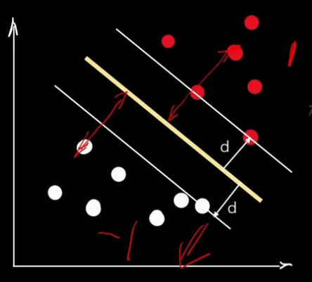
??????? 三个概念：

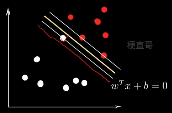
??????? 支持向量 support vector —— 距离决策边界最近的点

??????? 超平面 hyperplane —— “隔离带”中间的平分线

??????? 间隔 margin —— 最大化margin

????????

??????? 民主集中的思想 ~

?

????????

---

?

2、线性SVM —— 硬间隔 Hard Margin

?

?（假定数据本身线性可分）

??????? 通过上一小节我们得到优化目标：

??????? 最大化间隔margin 也就是 最大化距离 d，也就是点到超平面的垂直距离。

??????? 注意此处的距离和线性模型中的距离不同，线性模型中的距离是 yhat-y （斜边）

????????

?

??????? SVM的求解过程和线性方程一样：

??????????????? 先假设一个超平面，

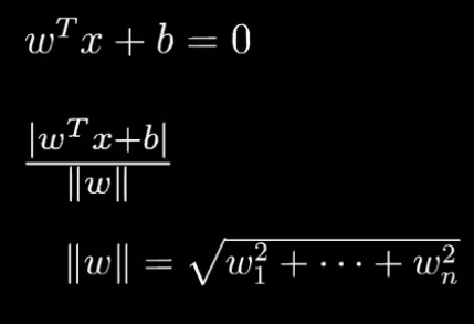
??????????????? 这里的W和X都是高维向量，点到高维空间中的距离有现成公式可以套用：

??????????????? ||w||为w的范数，表示高维空间中长度的概念。

????????????????

??????????????? 有了这样一个距离公式，隔离带就可以表示为一个分段函数的形式。

????????????????我们用1和-1来表示两个类别：

????????????????

????????????????

??????????????? 现在我们给柿子两边同时除以d 变形，再继续整理做变量代换：

???????????????

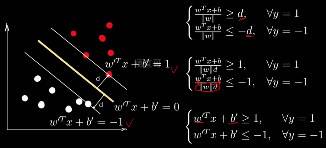
??????????????? 为了方便表示，看着撇多难受，我们再用w和b换回去，

????????????????但此时的w b和一开始推到时的w b，理论上已经不是同一个数了。

????????????????但是存在一个比例关系。在做一个变形：

????????????????

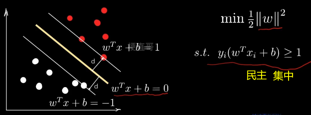
??????????????? 则现在的问题就简化为：

????????????????

???????????????? 这是一个不等式约束的最优化问题。梯度下降只能用于无约束的最优化。

???? ?? ???????? ps：

???????????? ? ? 不等式约束最优化 引入 松弛变量 到等式约束最优化。

???????? ? ????? 等式约束最优化 引入 拉格朗日乘子 到无约束最优化。

?

????????注意，这里的 i 是遍历所有的数据点。但在最小化范数时，我们只用到了支持向量。

????????

???????? 但是如果你相信的人也出了问题呢？

---

?

3、线性SVM —— 软间隔 Soft Margin

??????? 软间隔要解决的问题：

??????????????? 异常值 outliner??????

??????????????? 支持向量的选择、民主集中思想的弱点

????????????????

??????? 则需：建立容错机制，提升泛化能力

??????? 那么体现在数学上：允许点越过线一点点 ~

????????

??????? 那么怎么保证 这个减去的值不能太大呢？

????????

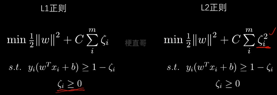
??????? 也就是说尽量让所有数据容错值的和最小。让二者取一个平衡。

??????? C 就是一个新的超参数，用来调节两者的权重值。

?

??????? 再看一下这个求和的形式，是不是特别像正则化？其实就可以看成正则化。

????????正则化项是一次的，所以叫L1正则。这里省略了绝对值符号，因为其就是正数。

????????

?

---

?

?4、线性SVM代码实现

?

数据集

import numpy as np
import matplotlib.pyplot as plt

from sklearn.datasets import make_blobs
x, y = make_blobs(
    n_samples=40, 
    centers=2, 
    random_state=0
)

plt.scatter(x[:,0], x[:,1], c = y)
plt.show()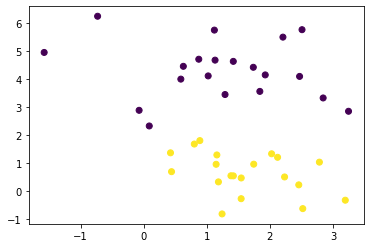

?

sklearn中的线性SVM

from sklearn.svm import LinearSVC

clf = LinearSVC(C = 1)

clf.fit(x, y)

LinearSVC

LinearSVC(C=1)

clf.score(x, y)

1.0

def decision_boundary_plot(X, y, clf):
    axis_x1_min, axis_x1_max = X[:,0].min() - 1, X[:,0].max() + 1
    axis_x2_min, axis_x2_max = X[:,1].min() - 1, X[:,1].max() + 1
    
    x1, x2 = np.meshgrid( np.arange(axis_x1_min,axis_x1_max, 0.01) , np.arange(axis_x2_min,axis_x2_max, 0.01))
    z = clf.predict(np.c_[x1.ravel(),x2.ravel()])
    z = z.reshape(x1.shape)
    
    from matplotlib.colors import ListedColormap
    custom_cmap = ListedColormap(['#F5B9EF','#BBFFBB','#F9F9CB'])

    plt.contourf(x1, x2, z, cmap=custom_cmap)
    plt.scatter(X[:,0], X[:,1], c=y)
    plt.show()

decision_boundary_plot(x, y, clf)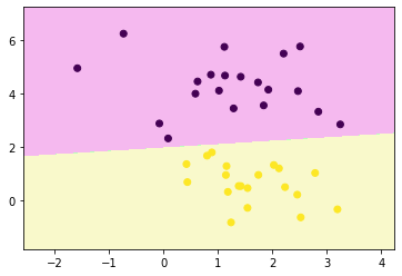

def plot_svm_margin(x, y, clf, ax = None):
    from sklearn.inspection import DecisionBoundaryDisplay
    DecisionBoundaryDisplay.from_estimator(
        clf,
        x,
        ax = ax,
        grid_resolution=50,
        plot_method="contour",
        colors="k",
        levels=[-1, 0, 1],
        alpha=0.5,
        linestyles=["--", "-", "--"],
    )
    plt.scatter(x[:,0], x[:,1], c = y)

plot_svm_margin(x, y, clf)
plt.show()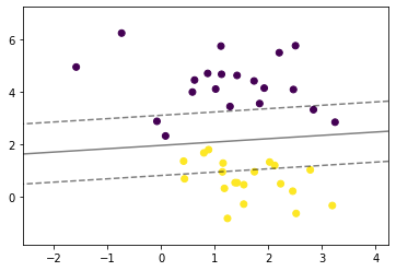

plt.rcParams["figure.figsize"] = (12, 8)

params = [0.1, 1, 10, 100]
for i, c in enumerate(params):
    clf = LinearSVC(C = c, random_state=0)
    clf.fit(x, y)
    
    ax = plt.subplot(2, 2, i + 1)
    plt.title("C: {0}".format(c))
    plot_svm_margin(x, y, clf, ax)
    
plt.show()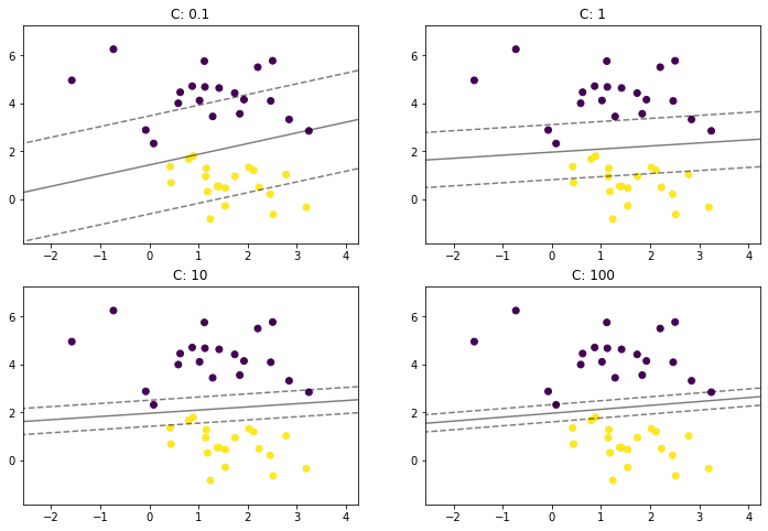

?

多分类

from sklearn import datasets

iris = datasets.load_iris()
x = iris.data
y = iris.target

注意SVM中只支持ovr ~

clf = LinearSVC(C = 0.1, multi_class='ovr', random_state=0)
clf.fit(x, y)

LinearSVC

LinearSVC(C=0.1, random_state=0)

clf.predict(x)

array([0, 0, 0, 0, 0, 0, 0, 0, 0, 0, 0, 0, 0, 0, 0, 0, 0, 0, 0, 0, 0, 0,
       0, 0, 0, 0, 0, 0, 0, 0, 0, 0, 0, 0, 0, 0, 0, 0, 0, 0, 0, 0, 0, 0,
       0, 0, 0, 0, 0, 0, 1, 1, 1, 1, 1, 1, 1, 1, 1, 1, 1, 1, 1, 1, 1, 1,
       2, 1, 1, 1, 2, 1, 1, 1, 1, 1, 1, 1, 1, 1, 1, 1, 1, 2, 2, 2, 1, 1,
       1, 1, 1, 1, 1, 1, 1, 1, 1, 1, 1, 1, 2, 2, 2, 2, 2, 2, 2, 2, 2, 2,
       2, 2, 2, 2, 2, 2, 2, 2, 2, 2, 2, 2, 2, 2, 2, 2, 2, 2, 2, 1, 2, 2,
       2, 2, 2, 2, 2, 2, 2, 2, 2, 2, 2, 2, 2, 2, 2, 2, 2, 2])

?

---

?

?5、非线性SVM —— 核技巧

?

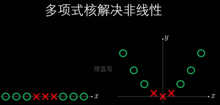
线性不可分问题

????????

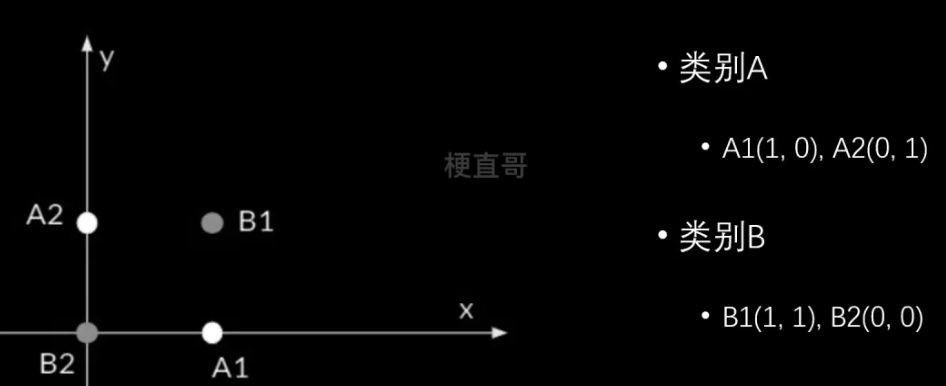
???????? 升维映射

????????

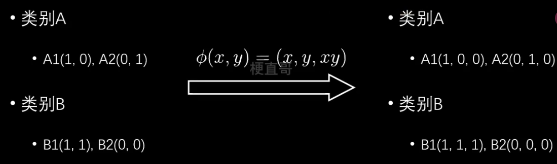
??????? 高维线性可分

????????

?????? 已经有前人在数学上证明：

??????? 如果原始的空间是有限的，也就是说特征数是有限的，

????????那么一定存在一个高位的特征空间能够分割这些样本。

????????

软间隔对偶 dual 问题?

????????

??????? 则现在就要解决右边的问题。

?????????

??????? 套上一个 φ 就可以升维，但是可能会导致维度灾难，所以就要使用核函数。

????????

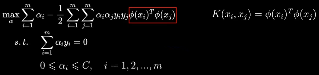
常用的核函数

????????

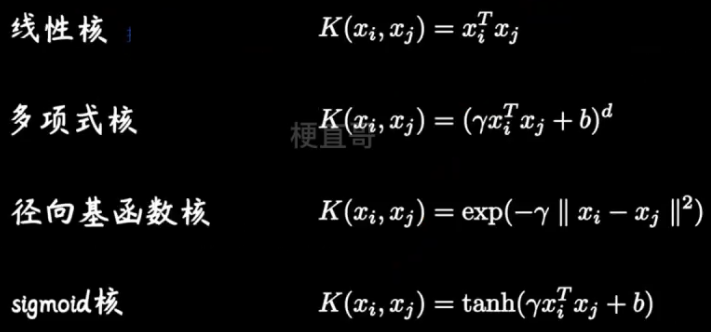
??????? 他们就像一个武器套装，能够方便针对软间隔对偶问题实现升维操作。

?那么为什么升维就能解决不可分的问题呢？

??????? 希尔伯特空间的元素是函数，因此可以看成无穷维度的向量。

????????

?

?核技巧的作用

??????? 映射到高维空间

??????? 大大减少了计算量，尤其是对于高维向量的相乘操作，同时也不需要额外存储中间的结果

??????? 不仅限于SVM，实际上 只要存在着 xi ，xj 的最优化问题。

????????

?

---

?

?6、非线性SVM —— 核函数

?

多项式核函数

?????????

????????以下将说明，为什么这个核函数相当于引入了多项式的特征。

??????? 为了推导方便，此处使用x，y

????????????????

????????????????

????????

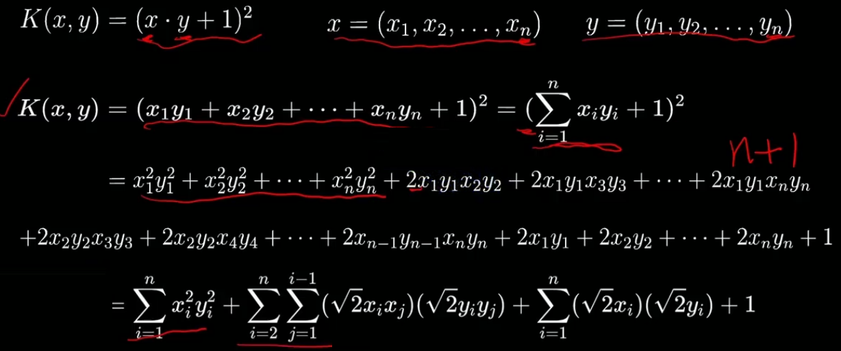
高斯核函数

????????

??????? 也叫 RBF核函数、径向基函数

??????? Radial Basic Function Kernel

????????

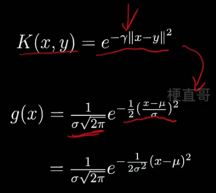
??????? 则根据下图可知，当 γ 越大的时候，映射的高斯函数就越发陡峭。

????????????????

??????? 在做高斯核映射时，需要选择地标。也就是下图中公式里的 y。

????????

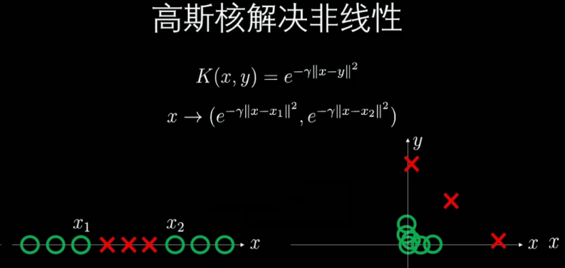
??????? 每个数据点都可以当做地标。

??????? 所以有多少个数据就会映射出多少个维度。

??????? 假定现在有m个维度为n的数据，则高斯核就可以将其映射成mxm维的数据。

??????? 当m非常大的时候，高斯核的运算效率其实很低，但当m并不大甚至小于n的时候，使用核函数就会变得非常高效了。（？存疑 小于）

?

---

?

?7、非线性SVM代码实现

?

如何选择核函数？

当特征多且接近样本数量，可直接选择线性核SVM。

当特征数少，样本数正常，推荐选用高斯核函数。

当特征数少，样本数很大，建议选择多项式核函数，切记阶数不能过高，否则复杂度过高，难以计算。

?

多项式特征解决非线性问题

import numpy as np
import matplotlib.pyplot as plt

from sklearn.datasets import make_moons
x, y = make_moons(n_samples=100, noise=0.2, random_state=0)

plt.scatter(x[:,0], x[:,1], c = y)
plt.show()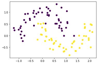

from sklearn.svm import LinearSVC

lsvc = LinearSVC()
lsvc.fit(x,y)

LinearSVC

LinearSVC()

def decision_boundary_plot(X, y, clf):
    axis_x1_min, axis_x1_max = X[:,0].min() - 1, X[:,0].max() + 1
    axis_x2_min, axis_x2_max = X[:,1].min() - 1, X[:,1].max() + 1
    
    x1, x2 = np.meshgrid( np.arange(axis_x1_min,axis_x1_max, 0.01) , np.arange(axis_x2_min,axis_x2_max, 0.01))
    z = clf.predict(np.c_[x1.ravel(),x2.ravel()])
    z = z.reshape(x1.shape)
    
    from matplotlib.colors import ListedColormap
    custom_cmap = ListedColormap(['#F5B9EF','#BBFFBB','#F9F9CB'])

    plt.contourf(x1, x2, z, cmap=custom_cmap)
    plt.scatter(X[:,0], X[:,1], c=y)
    plt.show()

decision_boundary_plot(x,y,lsvc)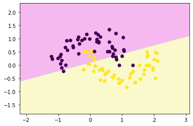

from sklearn.preprocessing import PolynomialFeatures, StandardScaler
from sklearn.pipeline import Pipeline

poly_svc = Pipeline([
    ("poly", PolynomialFeatures(degree=3)),
    ("std_scaler", StandardScaler()),
    ("linearSVC", LinearSVC())
])

poly_svc.fit(x,y)

Pipeline

Pipeline(steps=[('poly', PolynomialFeatures(degree=3)),
                ('std_scaler', StandardScaler()), ('linearSVC', LinearSVC())])

PolynomialFeatures

PolynomialFeatures(degree=3)

StandardScaler

StandardScaler()

LinearSVC

LinearSVC()

decision_boundary_plot(x,y,poly_svc)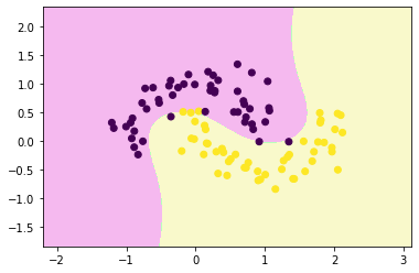

?

核函数解决非线性问题

from sklearn.svm import SVC

poly_svc = Pipeline([
    ("std_scaler", StandardScaler()),
    ("polySVC", SVC(kernel='poly', degree=3, coef0=5 ))
])
poly_svc.fit(x,y)

Pipeline

Pipeline(steps=[('std_scaler', StandardScaler()),
                ('polySVC', SVC(coef0=5, kernel='poly'))])

StandardScaler

StandardScaler()

SVC

SVC(coef0=5, kernel='poly')

decision_boundary_plot(x,y,poly_svc)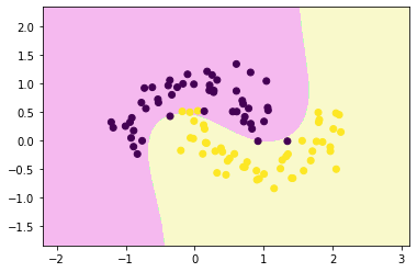

rbf_svc = Pipeline([
    ("std_scaler", StandardScaler()),
    ("rbfSVC", SVC(kernel='rbf', gamma=0.1 ))
])
rbf_svc.fit(x,y)
decision_boundary_plot(x,y,rbf_svc)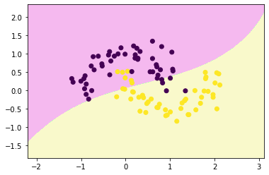

rbf_svc = Pipeline([
    ("std_scaler", StandardScaler()),
    ("rbfSVC", SVC(kernel='rbf', gamma=10 ))
])
rbf_svc.fit(x,y)
decision_boundary_plot(x,y,rbf_svc)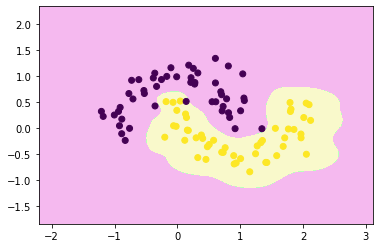

rbf_svc = Pipeline([
    ("std_scaler", StandardScaler()),
    ("rbfSVC", SVC(kernel='rbf', gamma=100 ))
])
rbf_svc.fit(x,y)
decision_boundary_plot(x,y,rbf_svc)

?

---

?

?8、SVM解决回归任务

?

?????????

????????

?????????

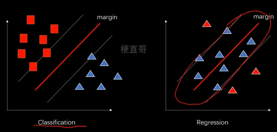
import numpy as np
import matplotlib.pyplot as plt

np.random.seed(666)
x = np.random.uniform(-3,3,size=100)
y = 0.5 * x**2 +x +2 +np.random.normal(0,1,size=100)
X = x.reshape(-1,1)

plt.scatter(x,y)
plt.show()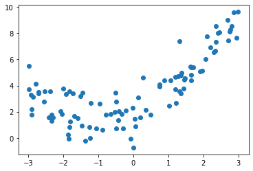

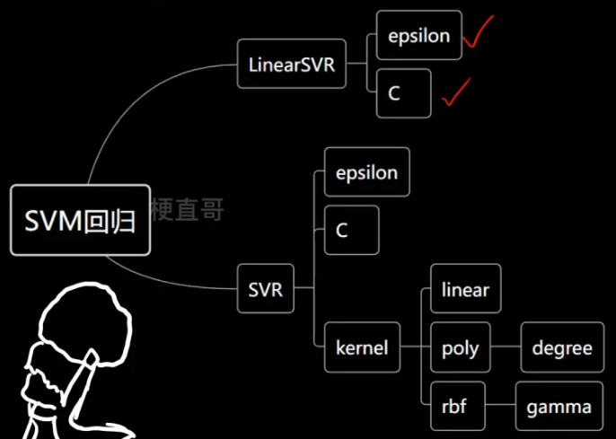
from sklearn.svm import LinearSVR
from sklearn.preprocessing import StandardScaler
from sklearn.pipeline import Pipeline

def StandardLinearSVR(epsilon=0.1):
    return Pipeline([
        ("std_scaler",StandardScaler()),
        ("linearSVR",LinearSVR(epsilon=epsilon))
    ])

svr = StandardLinearSVR()
svr.fit(X,y)
y_predict = svr.predict(X)
plt.scatter(x,y)
plt.plot(np.sort(x),y_predict[np.argsort(x)],color='r')
plt.show()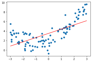

svr.score(X,y)

0.48764762540009954

from sklearn.svm import SVR

def StandardSVR(epsilon=0.1):
    return Pipeline([
        ('std_scaler',StandardScaler())
        ,('SVR',SVR(kernel='rbf',epsilon=epsilon))
    ])

svr = StandardSVR()
svr.fit(X,y)
y_predict = svr.predict(X)
plt.scatter(x,y)
plt.plot(np.sort(x),y_predict[np.argsort(x)],color='r')
plt.show()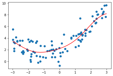

svr.score(X,y)

0.8138647789256847