吴恩达深度学习L1W4作业2

深度神经网络应用--图像分类

完成此作业后，你将完成第4周最后的编程任务，也是本课程最后的编程任务！

你将使用在上一个作业中实现的函数来构建深层网络，并将其应用于分类cat图像和非cat图像。 希望你会看到相对于先前的逻辑回归实现的分类，准确性有所提高。

完成此任务后，你将能够：

• 建立深度神经网络并将其应用于监督学习。

让我们开始吧！

1 安装包

让我们首先导入在作业过程中需要的所有软件包。

• numpy是Python科学计算的基本包。
• matplotlib?是在Python中常用的绘制图形的库。
• h5py是一个常用的包，可以处理存储为H5文件格式的数据集
• 这里最后通过PIL和?scipy用你自己的图片去测试模型效果。
• dnn_app_utils提供了上一作业教程“逐步构建你的深度神经网络”中实现的函数。
• np.random.seed（1）使所有随机函数调用保持一致。 这将有助于我们评估你的作业。

cd ../input/deeplearning46278
/home/kesci/input/deeplearning46278

import time
import numpy as np
import h5py
import matplotlib.pyplot as plt
import scipy
from PIL import Image
from scipy import ndimage
from dnn_app_utils_v2 import *

%matplotlib inline
plt.rcParams['figure.figsize'] = (5.0, 4.0) # set default size of plots
plt.rcParams['image.interpolation'] = 'nearest'
plt.rcParams['image.cmap'] = 'gray'

%load_ext autoreload
%autoreload 2

np.random.seed(1)

2 数据集

你将使用与“用神经网络思想实现Logistic回归”（作业2）中相同的“cats vs non-cats”数据集。 此前你建立的模型在对猫和非猫图像进行分类时只有70％的准确率。 希望你的新模型会更好！

问题说明：你将获得一个包含以下内容的数据集（"data.h5"）：
???? - 标记为cat（1）和非cat（0）图像的训练集m_train
???? - 标记为cat或non-cat图像的测试集m_test
???? - 每个图像的维度都为（num_px，num_px，3），其中3表示3个通道（RGB）。

让我们熟悉一下数据集吧， 首先通过运行以下代码来加载数据。

train_x_orig, train_y, test_x_orig, test_y, classes = load_data()

?运行以下代码以展示数据集中的图像。 通过更改索引，然后重新运行单元以查看其他图像。

# Example of a picture
index = 7
plt.imshow(train_x_orig[index])
print ("y = " + str(train_y[0,index]) + ". It's a " + classes[train_y[0,index]].decode("utf-8") +  " picture.")

?

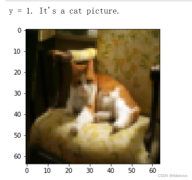
# Explore your dataset 
m_train = train_x_orig.shape[0]
num_px = train_x_orig.shape[1]
m_test = test_x_orig.shape[0]

print ("Number of training examples: " + str(m_train))
print ("Number of testing examples: " + str(m_test))
print ("Each image is of size: (" + str(num_px) + ", " + str(num_px) + ", 3)")
print ("train_x_orig shape: " + str(train_x_orig.shape))
print ("train_y shape: " + str(train_y.shape))
print ("test_x_orig shape: " + str(test_x_orig.shape))
print ("test_y shape: " + str(test_y.shape))

?

与往常一样，在将图像输入到网络之前，需要对图像进行重塑和标准化。 下面单元格给出了相关代码。

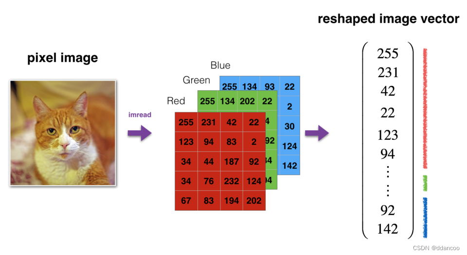
# Reshape the training and test examples 
train_x_flatten = train_x_orig.reshape(train_x_orig.shape[0], -1).T   # The "-1" makes reshape flatten the remaining dimensions
test_x_flatten = test_x_orig.reshape(test_x_orig.shape[0], -1).T

# Standardize data to have feature values between 0 and 1.
train_x = train_x_flatten/255.
test_x = test_x_flatten/255.

print ("train_x's shape: " + str(train_x.shape))
print ("test_x's shape: " + str(test_x.shape))

?

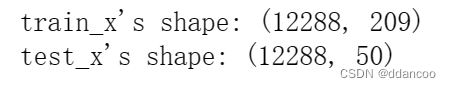
?12,288等于64×64×364×64×3，这是图像重塑为向量的大小。

3 模型的结构

?

现在你已经熟悉了数据集，是时候建立一个深度神经网络来区分猫图像和非猫图像了。

你将建立两个不同的模型：

• 2层神经网络
• L层深度神经网络

然后，你将比较这些模型的性能，并尝试不同的L值。

让我们看一下两种架构。

3.1 2层神经网络

图2：2层神经网络。

该模型可以总结为：INPUT -> LINEAR -> RELU -> LINEAR -> SIGMOID -> OUTPUT

图2的详细架构：

• 输入维度为（64,64,3）的图像，将其展平为大小为（12288,1）的向量。
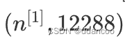• 相应的向量：乘以大小为的权重矩阵。
• 然后添加一个偏差项并按照公式获得以下向量：。
• 然后，重复相同的过程。
• 将所得向量乘以并加上截距（偏差）。
• 最后，采用结果的sigmoid值。 如果大于0.5，则将其分类为猫。

3.2 L层深度神经网络

用上面的方式很难表示一个L层的深度神经网络。 这是一个简化的网络表示形式：

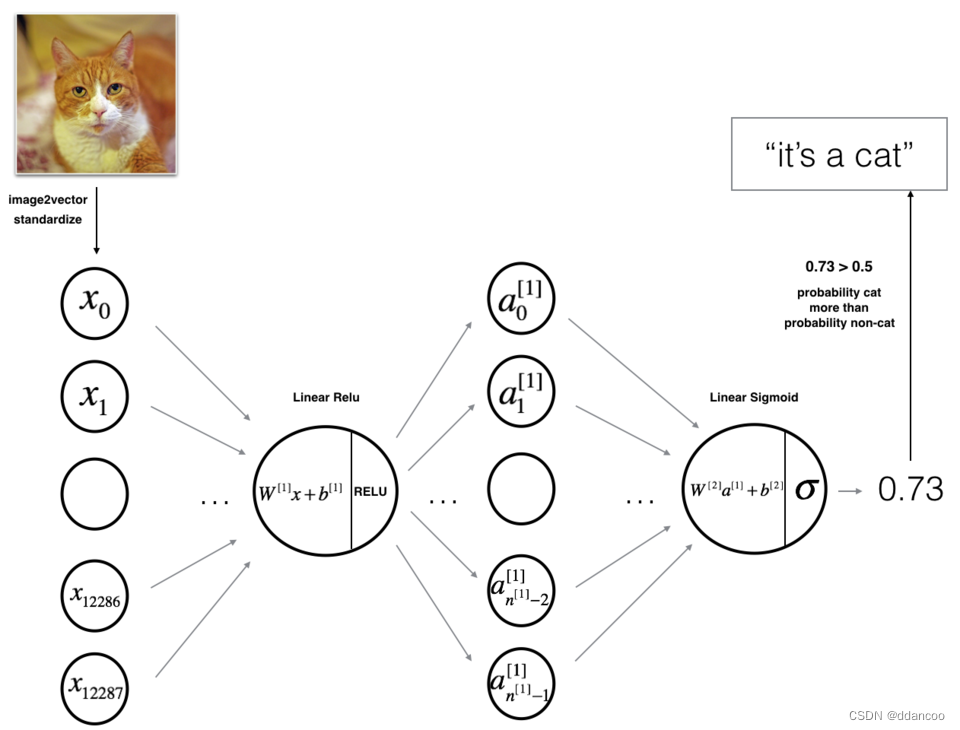
图3：L层神经网络。
该模型可以总结为：[LINEAR -> RELU]?×?(L-1) -> LINEAR -> SIGMOID

图3的详细结构：

• 输入维度为（64,64,3）的图像，将其展平为大小为（12288,1）的向量。
• 相应的向量：乘以权重矩阵，然后加上截距，结果为线性单位。
• 接下来计算获得的线性单元。对于每个()，可以重复数次，具体取决于模型体系结构。
• 最后，采用最终线性单位的sigmoid值。如果大于0.5，则将其分类为猫。

3.3 通用步骤

与往常一样，你将遵循深度学习步骤来构建模型：
????1.初始化参数/定义超参数
????2.循环num_iterations次：
????????a. 正向传播
????????b. 计算损失函数
????????C. 反向传播
????????d. 更新参数（使用参数和反向传播的梯度）
????4.使用训练好的参数来预测标签

现在让我们实现这两个模型！

4 两层神经网络

问题：使用你在上一个作业中实现的辅助函数来构建具有以下结构的2层神经网络：LINEAR -> RELU -> LINEAR -> SIGMOID，你可能需要的函数及其输入为：

def initialize_parameters(n_x, n_h, n_y):  
    ...  
    return parameters   
def linear_activation_forward(A_prev, W, b, activation):  
    ...  
    return A, cache  
def compute_cost(AL, Y):  
    ...  
    return cost  
def linear_activation_backward(dA, cache, activation):  
    ...  
    return dA_prev, dW, db  
def update_parameters(parameters, grads, learning_rate):  
    ...  
    return parameters

### CONSTANTS DEFINING THE MODEL ####
n_x = 12288     # num_px * num_px * 3
n_h = 7
n_y = 1
layers_dims = (n_x, n_h, n_y)

# GRADED FUNCTION: two_layer_model

def two_layer_model(X, Y, layers_dims, learning_rate = 0.0075, num_iterations = 3000, print_cost=False):
    """
    Implements a two-layer neural network: LINEAR->RELU->LINEAR->SIGMOID.
    
    Arguments:
    X -- input data, of shape (n_x, number of examples)
    Y -- true "label" vector (containing 0 if cat, 1 if non-cat), of shape (1, number of examples)
    layers_dims -- dimensions of the layers (n_x, n_h, n_y)
    num_iterations -- number of iterations of the optimization loop
    learning_rate -- learning rate of the gradient descent update rule
    print_cost -- If set to True, this will print the cost every 100 iterations 
    
    Returns:
    parameters -- a dictionary containing W1, W2, b1, and b2
    """
    
    np.random.seed(1)
    grads = {}
    costs = []                              # to keep track of the cost
    m = X.shape[1]                           # number of examples
    (n_x, n_h, n_y) = layers_dims
    
    # Initialize parameters dictionary, by calling one of the functions you'd previously implemented
    ### START CODE HERE ### (≈ 1 line of code)

    parameters=initialize_parameters(n_x,n_h,n_y)
    
    ### END CODE HERE ###
    
    # Get W1, b1, W2 and b2 from the dictionary parameters.
    W1 = parameters["W1"]
    b1 = parameters["b1"]
    W2 = parameters["W2"]
    b2 = parameters["b2"]
    
    # Loop (gradient descent)

    for i in range(0, num_iterations):

        # Forward propagation: LINEAR -> RELU -> LINEAR -> SIGMOID. Inputs: "X, W1, b1". Output: "A1, cache1, A2, cache2".
        ### START CODE HERE ### (≈ 2 lines of code)

        A1,cache1=linear_activation_forward(X,W1,b1,activation="relu")
        A2,cache2=linear_activation_forward(A1,W2,b2,activation="sigmoid")
        
        ### END CODE HERE ###
        
        # Compute cost
        ### START CODE HERE ### (≈ 1 line of code)
        
        cost=compute_cost(A2,Y)

        ### END CODE HERE ###
        
        # Initializing backward propagation
        dA2 = - (np.divide(Y, A2) - np.divide(1 - Y, 1 - A2))
        
        # Backward propagation. Inputs: "dA2, cache2, cache1". Outputs: "dA1, dW2, db2; also dA0 (not used), dW1, db1".
        ### START CODE HERE ### (≈ 2 lines of code)

        dA1,dW2,db2=linear_activation_backward(dA2,cache2,activation="sigmoid")
        dA0,dW1,db1=linear_activation_backward(dA1,cache1,activation="relu")
        
        ### END CODE HERE ###
        
        # Set grads['dWl'] to dW1, grads['db1'] to db1, grads['dW2'] to dW2, grads['db2'] to db2
        grads['dW1'] = dW1
        grads['db1'] = db1
        grads['dW2'] = dW2
        grads['db2'] = db2
        
        # Update parameters.
        ### START CODE HERE ### (approx. 1 line of code)

        parameters=update_parameters(parameters,grads,learning_rate)
        ### END CODE HERE ###

        # Retrieve W1, b1, W2, b2 from parameters
        W1 = parameters["W1"]
        b1 = parameters["b1"]
        W2 = parameters["W2"]
        b2 = parameters["b2"]
        
        # Print the cost every 100 training example
        if print_cost and i % 100 == 0:
            print("Cost after iteration {}: {}".format(i, np.squeeze(cost)))
        if print_cost and i % 100 == 0:
            costs.append(cost)
       
    # plot the cost

    plt.plot(np.squeeze(costs))
    plt.ylabel('cost')
    plt.xlabel('iterations (per tens)')
    plt.title("Learning rate =" + str(learning_rate))
    plt.show()
    
    return parameters

parameters = two_layer_model(train_x, train_y, layers_dims = (n_x, n_h, n_y), num_iterations = 2500, print_cost=True)

?

你构建了向量化的实现！ 否则，可能需要花费10倍的时间来训练它。

你可以使用训练好的参数对数据集中的图像进行分类。 要查看训练和测试集的预测结果，请运行以下单元格。

??

?

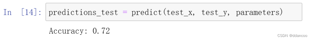
注意：你可能会注意到，以较少的迭代次数（例如1500）运行模型可以使测试集具有更高的准确性。 这称为“尽早停止”，我们将在下一课程中讨论。 提前停止是防止过拟合的一种方法。

恭喜你！看来你的2层神经网络的性能（72％）比逻辑回归实现（70％，第2周的作业）更好。 让我们看看使用L层模型是否可以做得更好。

5 L层神经网络

问题：使用之前实现的辅助函数来构建具有以下结构的L层神经网络：[LINEAR -> RELU]×(L-1) -> LINEAR -> SIGMOID。 你可能需要的函数及其输入为：

def initialize_parameters_deep(layer_dims):  
    ...  
    return parameters   
def L_model_forward(X, parameters):  
    ...  
    return AL, caches  
def compute_cost(AL, Y):  
    ...  
    return cost  
def L_model_backward(AL, Y, caches):  
    ...  
    return grads  
def update_parameters(parameters, grads, learning_rate):  
    ...  
    return parameters

?

# GRADED FUNCTION: L_layer_model

def L_layer_model(X, Y, layers_dims, learning_rate = 0.0075, num_iterations = 3000, print_cost=False):#lr was 0.009
    """
    Implements a L-layer neural network: [LINEAR->RELU]*(L-1)->LINEAR->SIGMOID.
    
    Arguments:
    X -- data, numpy array of shape (number of examples, num_px * num_px * 3)
    Y -- true "label" vector (containing 0 if cat, 1 if non-cat), of shape (1, number of examples)
    layers_dims -- list containing the input size and each layer size, of length (number of layers + 1).
    learning_rate -- learning rate of the gradient descent update rule
    num_iterations -- number of iterations of the optimization loop
    print_cost -- if True, it prints the cost every 100 steps
    
    Returns:
    parameters -- parameters learnt by the model. They can then be used to predict.
    """

    np.random.seed(1)
    costs = []                         # keep track of cost
    
    # Parameters initialization.
    ### START CODE HERE ###

    parameters=initialize_parameters_deep(layers_dims)
    
    ### END CODE HERE ###
    
    # Loop (gradient descent)
    for i in range(0, num_iterations):

        # Forward propagation: [LINEAR -> RELU]*(L-1) -> LINEAR -> SIGMOID.
        ### START CODE HERE ### (≈ 1 line of code)
        
        AL,caches=L_model_forward(X,parameters)

        ### END CODE HERE ###
        
        # Compute cost.
        ### START CODE HERE ### (≈ 1 line of code)
        
        cost=compute_cost(AL,Y)

        ### END CODE HERE ###
    
        # Backward propagation.
        ### START CODE HERE ### (≈ 1 line of code)

        grads=L_model_backward(AL,Y,caches
                              )
        ### END CODE HERE ###
 
        # Update parameters.
        ### START CODE HERE ### (≈ 1 line of code)
        
        parameters=update_parameters(parameters,grads,learning_rate)

        ### END CODE HERE ###
                
        # Print the cost every 100 training example
        if print_cost and i % 100 == 0:
            print ("Cost after iteration %i: %f" %(i, cost))
        if print_cost and i % 100 == 0:
            costs.append(cost)
            
    # plot the cost
    plt.plot(np.squeeze(costs))
    plt.ylabel('cost')
    plt.xlabel('iterations (per tens)')
    plt.title("Learning rate =" + str(learning_rate))
    plt.show()
    
    return parameters

parameters = L_layer_model(train_x, train_y, layers_dims, num_iterations = 2500, print_cost = True)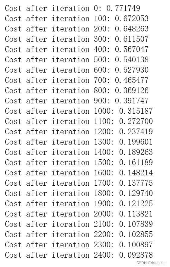

pred_train = predict(train_x, train_y, parameters)

?

pred_test = predict(test_x, test_y, parameters)

?

Good！在相同的测试集上，你的5层的神经网络似乎比2层神经网络具有更好的性能（80％）。做的好！

在下一作业教程“改善深度神经网络”中，你将学习如何通过系统地匹配更好的超参数（学习率，层数，迭代次数以及下一门课程中还将学习到的其他参数）来获得更高的准确性。

?6 结果分析

首先，让我们看一下L层模型标记错误的一些图像。 这将显示一些分类错误的图像。

print_mislabeled_images(classes, test_x, test_y, pred_test)

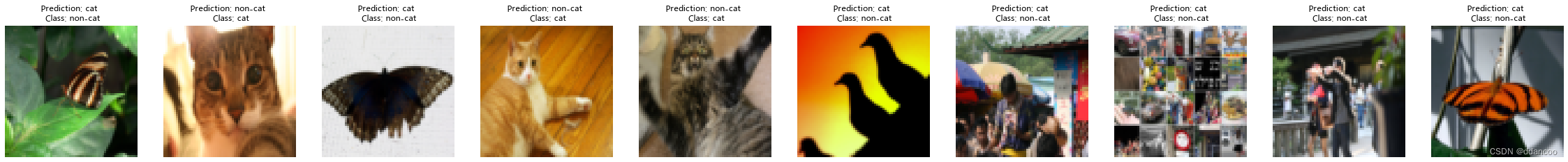
该模型在表现效果较差的的图像包括：

• 猫身处于异常位置
• 图片背景与猫颜色类似
• 猫的种类和颜色稀有
• 相机角度
• 图片的亮度
• 比例变化（猫的图像很大或很小）

7 使用你自己的图像进行测试（可选练习）

祝贺你完成此作业。 你可以使用自己的图像测试并查看模型的输出。要做到这一点：
???? 1.单击此笔记本上部栏中的“File”，然后单击“Open”以在Coursera Hub上运行。
???? 2.将图像添加到Jupyter Notebook的目录中，在“images”文件夹中
???? 3.在以下代码中更改图像的名称
???? 4.运行代码，检查算法是否正确（1 = cat，0 = non-cat）！

## START CODE HERE ##
my_image = "my_image.jpg" # change this to the name of your image file 
my_label_y = [1] # the true class of your image (1 -> cat, 0 -> non-cat)
## END CODE HERE ##

fname = my_image
image = np.array(plt.imread(fname))
my_image = np.array(Image.fromarray(image).resize(size=(num_px,num_px))).reshape((num_px*num_px*3,1))
my_predicted_image = predict(my_image, my_label_y, parameters)

plt.imshow(image)
print ("y = " + str(np.squeeze(my_predicted_image)) + ", your L-layer model predicts a \"" + classes[int(np.squeeze(my_predicted_image)),].decode("utf-8") +  "\" picture.")
Accuracy: 0.0
y = 0.0, your L-layer model predicts a "non-cat" pic

?