工具系列：PyCaret介绍_二分类模型

2023-12-21 18:03:15

👋 工具系列：PyCaret介绍_二分类模型

PyCaret是一个开源的、低代码的Python机器学习库，可以自动化机器学习工作流程。它是一个端到端的机器学习和模型管理工具，可以大大加快实验周期并提高工作效率。

与其他开源机器学习库相比，PyCaret是一个替代低代码库，可以用几行代码代替数百行代码。这使得实验速度指数级增加，效率更高。PyCaret本质上是围绕几个机器学习库和框架（如scikit-learn、XGBoost、LightGBM、CatBoost、spaCy、Optuna、Hyperopt、Ray等）的Python封装。

PyCaret的设计和简洁性受到了Gartner首次使用的公民数据科学家这一新兴角色的启发。公民数据科学家是能够执行简单和中等复杂的分析任务的高级用户，而以前这些任务需要更多的技术专业知识。

💻 安装

PyCaret在以下64位系统上进行了测试和支持：

Python 3.7 - 3.10
仅适用于Ubuntu的Python 3.9
Ubuntu 16.04或更高版本
Windows 7或更高版本

您可以使用Python的pip软件包管理器安装PyCaret：

pip install pycaret

PyCaret的默认安装不会自动安装所有额外的依赖项。为此，您需要安装完整版本：

pip install pycaret[full]

或者根据您的用例，您可以安装以下其中之一的变体：

pip install pycaret[analysis]
pip install pycaret[models]
pip install pycaret[tuner]
pip install pycaret[mlops]
pip install pycaret[parallel]
pip install pycaret[test]

# 导入pycaret库
import pycaret

# 打印pycaret库的版本号
pycaret.__version__

'3.0.0'

🚀 快速开始

PyCaret的分类模块是一个监督学习模块，用于将元素分类到不同的组中。其目标是预测离散且无序的分类标签。

一些常见的用例包括预测客户是否违约（是或否）、预测客户流失（客户将离开或保留）、发现的疾病（阳性或阴性）。

该模块可用于二分类或多分类问题。它提供了几种预处理功能，通过设置函数对数据进行建模准备。它拥有超过18种可直接使用的算法和多个图表，用于分析训练模型的性能。

在PyCaret中，典型的工作流程按照以下5个步骤进行：

设置 ?? 比较模型 ?? 分析模型 ?? 预测 ?? 保存模型

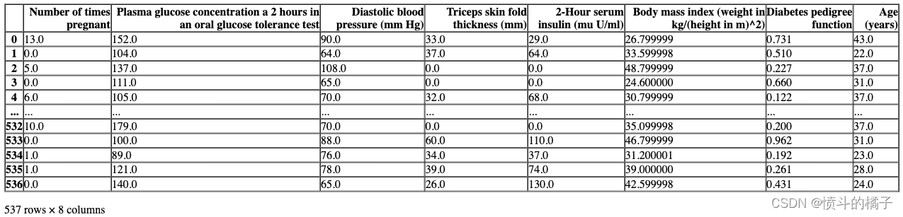
# 从pycaret数据集模块加载示例数据集
from pycaret.datasets import get_data
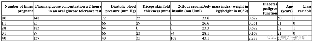
data = get_data('diabetes')

在这里插入图片描述

设置

此函数初始化训练环境并创建转换流水线。在执行PyCaret中的任何其他函数之前，必须调用设置函数。它只有两个必需的参数，即data和target。所有其他参数都是可选的。

# 导入pycaret分类模块和初始化设置
from pycaret.classification import *

# 初始化设置
# data: 数据集，包含特征和目标变量
# target: 目标变量的名称
# session_id: 设置随机种子，用于复现结果
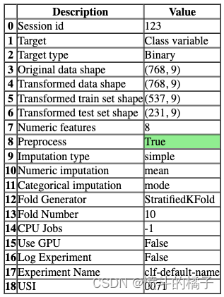
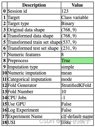
s = setup(data, target='Class variable', session_id=123)

在这里插入图片描述

一旦设置成功执行，它将显示包含实验级别信息的信息网格。

会话ID： 伪随机数，在所有函数中作为种子分布，以便以后可以重现。如果没有传递session_id，则会自动生成一个随机数，并分发给所有函数。
目标类型： 二进制、多类或回归。目标类型会自动检测。
标签编码： 当目标变量为字符串类型（例如’Yes’或’No’）而不是1或0时，它会自动将标签编码为1和0，并显示映射（0：No，1：Yes）以供参考。在本教程中，不需要进行标签编码，因为目标变量是数值类型。
原始数据形状： 在进行任何转换之前的原始数据形状。
转换后的训练集形状： 转换后的训练集形状
转换后的测试集形状： 转换后的测试集形状
数值特征： 被视为数值的特征数量。
分类特征： 被视为分类的特征数量。

PyCaret中有两组API供您使用。 (1) 函数式API（如上所示）和 (2) 面向对象的API。

使用面向对象的API时，您不会直接执行函数，而是导入一个类并执行类的方法。

# 导入ClassificationExperiment类并初始化该类
from pycaret.classification import ClassificationExperiment
exp = ClassificationExperiment()

# 检查exp的类型

type(exp)

pycaret.classification.oop.ClassificationExperiment

# 初始化设置实验
exp.setup(data, target='Class variable', session_id=123) 

# 参数说明：
# - data: 数据集，用于训练和测试模型
# - target: 目标变量，即我们要预测的变量
# - session_id: 实验的会话ID，用于复现实验结果

在这里插入图片描述

<pycaret.classification.oop.ClassificationExperiment at 0x2e24286edc0>

你可以使用任何一种方法，即函数式或面向对象编程，并且可以在两组API之间来回切换。选择的方法不会影响结果，并且已经进行了一致性测试。

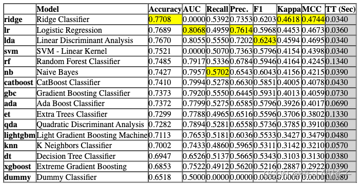
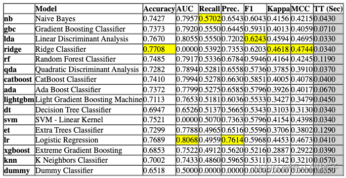
比较模型

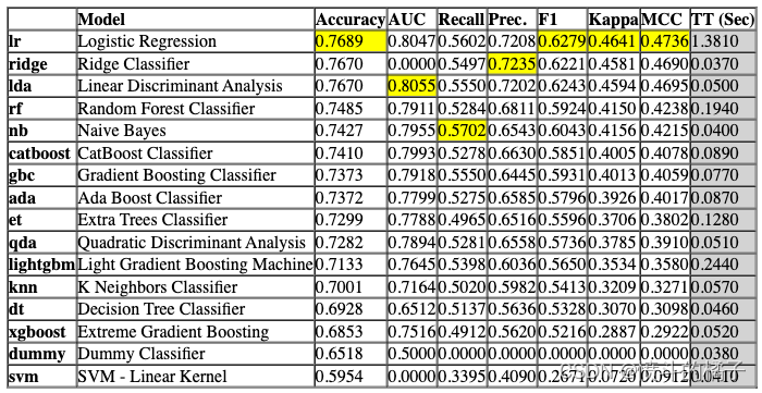
该函数使用交叉验证训练和评估模型库中所有可用的估计器的性能。该函数的输出是一个带有平均交叉验证分数的评分表。可以使用get_metrics函数访问CV期间评估的指标。可以使用add_metric和remove_metric函数添加或删除自定义指标。

# 比较基准模型

# 使用compare_models()函数比较不同的基准模型，该函数会自动选择最佳的模型

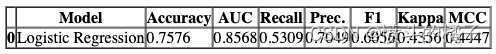
best = compare_models()

在这里插入图片描述

Processing:   0%|          | 0/69 [00:00<?, ?it/s]

# 比较模型
exp.compare_models()

在这里插入图片描述

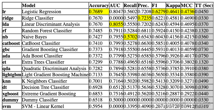
Processing:   0%|          | 0/69 [00:00<?, ?it/s]

在这里插入图片描述

注意，函数式API和面向对象API之间的输出是一致的。本笔记本中的其余函数将仅使用函数式API显示。

分析模型

您可以使用plot_model函数来分析训练模型在测试集上的性能。在某些情况下，可能需要重新训练模型。

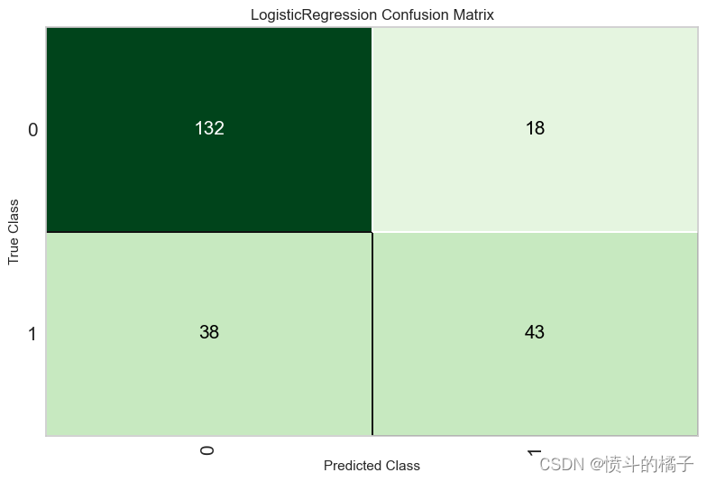
# 绘制混淆矩阵
# best是训练好的模型
# plot_model是一个函数，用于绘制模型的混淆矩阵
# 'confusion_matrix'是绘制混淆矩阵的参数
# 返回一个混淆矩阵图像
plot_model(best, plot='confusion_matrix')

在这里插入图片描述

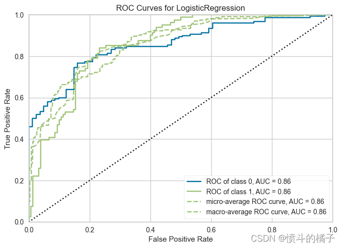
# 绘制模型的AUC曲线
# 参数best表示要绘制AUC曲线的模型
# 参数plot='auc'表示绘制AUC曲线
plot_model(best, plot='auc')

在这里插入图片描述

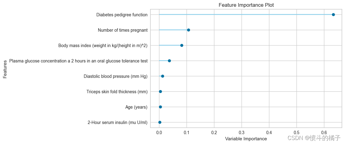
# 绘制特征重要性图
plot_model(model, plot='feature')

在这里插入图片描述

# 查询可使用的绘图功能
# help(plot_model)

An alternate to plot_model function is evaluate_model. It can only be used in Notebook since it uses ipywidget.

evaluate_model(best)

interactive(children=(ToggleButtons(description='Plot Type:', icons=('',), options=(('Pipeline Plot', 'pipelin…

预测

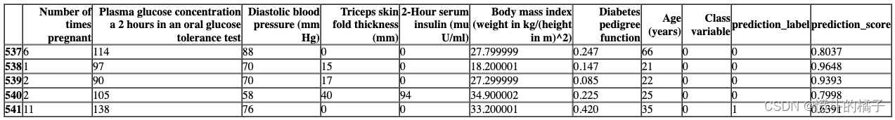
predict_model 函数会在数据框中返回 prediction_label 和 prediction_score（预测类别的概率）作为新的列。当数据为 None（默认值）时，它会使用在设置函数期间创建的测试集进行评分。

# 预测测试集数据
# 使用之前训练好的模型对测试集数据进行预测
holdout_pred = predict_model(best)

在这里插入图片描述

# 展示预测结果的数据框

# 使用head()函数显示数据框的前几行，默认显示前5行

holdout_pred.head()

在这里插入图片描述

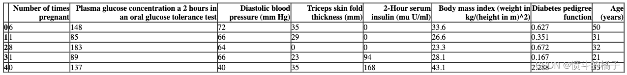
相同的函数适用于预测未见过的数据集上的标签。让我们创建原始数据的副本并删除Class variable。然后，我们可以使用没有标签的新数据框进行评分。

# 复制data，删除Class variable列

new_data = data.copy()
new_data.drop('Class variable', axis=1, inplace=True)
new_data.head()

在这里插入图片描述

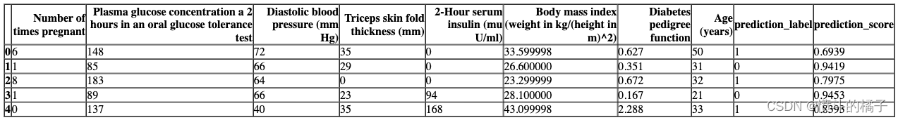
# 在新数据上预测模型
predictions = predict_model(best, data = new_data)
predictions.head()

在这里插入图片描述

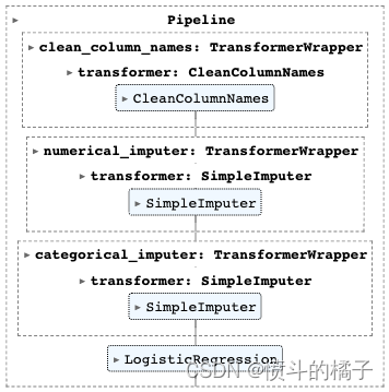
保存模型

最终我们可以使用save_model保存整个流水线

# save pipeline
save_model(best, 'my_first_pipeline')

Transformation Pipeline and Model Successfully Saved





(Pipeline(memory=FastMemory(location=C:\Users\owner\AppData\Local\Temp\joblib),
          steps=[('clean_column_names',
                  TransformerWrapper(exclude=None, include=None,
                                     transformer=CleanColumnNames(match='[\\]\\[\\,\\{\\}\\"\\:]+'))),
                 ('numerical_imputer',
                  TransformerWrapper(exclude=None,
                                     include=['Number of times pregnant',
                                              'Plasma glucose concentration a 2 '
                                              'hours in an oral glu...
                                                               fill_value=None,
                                                               missing_values=nan,
                                                               strategy='most_frequent',
                                                               verbose='deprecated'))),
                 ('trained_model',
                  LogisticRegression(C=1.0, class_weight=None, dual=False,
                                     fit_intercept=True, intercept_scaling=1,
                                     l1_ratio=None, max_iter=1000,
                                     multi_class='auto', n_jobs=None,
                                     penalty='l2', random_state=123,
                                     solver='lbfgs', tol=0.0001, verbose=0,
                                     warm_start=False))],
          verbose=False),
 'my_first_pipeline.pkl')

# 读取模型
loaded_best_pipeline = load_model('my_first_pipeline')
loaded_best_pipeline

Transformation Pipeline and Model Successfully Loaded

在这里插入图片描述

👇 详细的逐个函数概述

? 设置

setup 函数在 PyCaret 中初始化实验，并根据传入函数的所有参数创建转换流水线。在执行任何其他函数之前，必须调用 setup 函数。它有两个必需的参数：data 和 target。所有其他参数都是可选的，用于配置数据预处理流水线。

# 使用setup函数对数据进行预处理和设置
# 参数data表示要处理的数据
# 参数target表示目标变量的名称，即要预测的变量
# 参数session_id表示设置的会话ID，用于重现结果
s = setup(data, target = 'Class variable', session_id = 123)

在这里插入图片描述

要访问由设置函数创建的所有变量，例如转换后的数据集、随机状态等，您可以使用get_config方法。

# 获取所有可用的配置信息
get_config()

{'USI',
 'X',
 'X_test',
 'X_test_transformed',
 'X_train',
 'X_train_transformed',
 'X_transformed',
 '_available_plots',
 '_ml_usecase',
 'data',
 'dataset',
 'dataset_transformed',
 'exp_id',
 'exp_name_log',
 'fix_imbalance',
 'fold_generator',
 'fold_groups_param',
 'fold_shuffle_param',
 'gpu_n_jobs_param',
 'gpu_param',
 'html_param',
 'idx',
 'is_multiclass',
 'log_plots_param',
 'logging_param',
 'memory',
 'n_jobs_param',
 'pipeline',
 'seed',
 'target_param',
 'test',
 'test_transformed',
 'train',
 'train_transformed',
 'variable_and_property_keys',
 'variables',
 'y',
 'y_test',
 'y_test_transformed',
 'y_train',
 'y_train_transformed',
 'y_transformed'}

# 获取配置文件中的X_train_transformed数据
get_config('X_train_transformed')

在这里插入图片描述

# 打印当前的种子值
print("当前的种子值为: {}".format(get_config('seed')))

# 使用set_config函数来改变种子值
set_config('seed', 786)
# 打印新的种子值
print("新的种子值为: {}".format(get_config('seed')))

The current seed is: 123
The new seed is: 786

预处理配置和实验设置/参数都传递给setup函数。要查看所有可用参数，请检查docstring：

# help(setup)

# 初始化设置，使用normalize = True
s = setup(data, target = 'Class variable', session_id = 123,
          normalize = True, normalize_method = 'minmax')

在这里插入图片描述

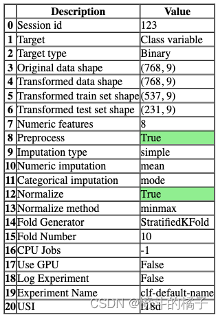
# 获取X_train_transformed的配置信息
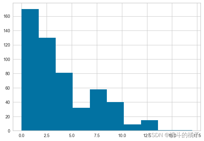
get_config('X_train_transformed')['Number of times pregnant'].hist()

<AxesSubplot:>

在这里插入图片描述

注意，所有的值都在0和1之间 - 这是因为我们在setup函数中传递了normalize=True。如果你不记得它与实际数据的比较方式，没问题 - 我们也可以使用get_config来访问非转换的值，然后进行比较。请参见下面的内容，并注意x轴上的值范围，并将其与上面的直方图进行比较。

# 获取配置文件中的训练数据集X_train的年龄列
get_config('X_train')['Number of times pregnant'].hist()

<AxesSubplot:>

在这里插入图片描述

? 比较模型

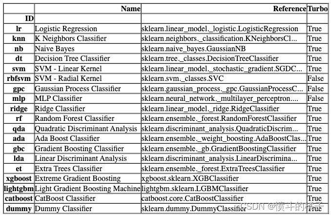
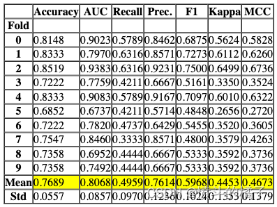
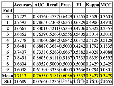
compare_models 函数使用交叉验证训练和评估模型库中所有可用的估计器的性能。该函数的输出是一个带有平均交叉验证分数的评分网格。可以使用 get_metrics 函数访问 CV 期间评估的指标。可以使用 add_metric 和 remove_metric 函数添加或删除自定义指标。

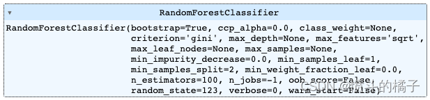
best = compare_models()

在这里插入图片描述

Processing:   0%|          | 0/69 [00:00<?, ?it/s]

compare_models默认使用模型库中的所有估计器（除了Turbo=False的模型）。要查看所有可用的模型，您可以使用函数models()。

# 调用函数来检查可用的模型
models()

在这里插入图片描述

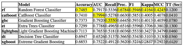
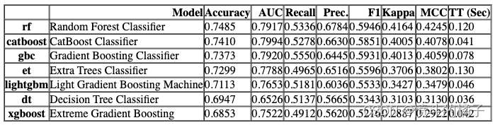
您可以在compare_models中使用include和exclude参数，只训练选择的模型或通过在exclude参数中传递模型id来排除特定模型的训练。

# 使用compare_models函数比较不同的决策树模型
compare_tree_models = compare_models(include = ['dt', 'rf', 'et', 'gbc', 'xgboost', 'lightgbm', 'catboost'])

在这里插入图片描述

Processing:   0%|          | 0/33 [00:00<?, ?it/s]

compare_tree_models

在这里插入图片描述

功能上面的函数返回训练好的模型对象作为输出。评分网格只显示，不返回。如果您需要访问评分网格，可以使用pull函数访问数据框。

compare_tree_models_results = pull()
compare_tree_models_results

在这里插入图片描述

默认情况下，compare_models函数返回基于sort参数中定义的指标的最佳性能模型。让我们修改我们的代码，返回基于MAE的前3个最佳模型。

# 导入所需的库
from pycaret.classification import compare_models

# 使用compare_models函数来比较不同模型的性能
# sort参数设置为'Recall'，表示按照召回率对模型进行排序
# n_select参数设置为3，表示选择排名前3的模型
best_recall_models_top3 = compare_models(sort='Recall', n_select=3)

在这里插入图片描述

Processing:   0%|          | 0/71 [00:00<?, ?it/s]

# 定义一个列表，用于存储Recall最高的前三个模型的名称
best_recall_models_top3

[GaussianNB(priors=None, var_smoothing=1e-09),
 GradientBoostingClassifier(ccp_alpha=0.0, criterion='friedman_mse', init=None,
                            learning_rate=0.1, loss='log_loss', max_depth=3,
                            max_features=None, max_leaf_nodes=None,
                            min_impurity_decrease=0.0, min_samples_leaf=1,
                            min_samples_split=2, min_weight_fraction_leaf=0.0,
                            n_estimators=100, n_iter_no_change=None,
                            random_state=123, subsample=1.0, tol=0.0001,
                            validation_fraction=0.1, verbose=0,
                            warm_start=False),
 LinearDiscriminantAnalysis(covariance_estimator=None, n_components=None,
                            priors=None, shrinkage=None, solver='svd',
                            store_covariance=False, tol=0.0001)]

一些在compare_models中可能非常有用的其他参数有：

fold
cross_validation
budget_time
errors
probability_threshold
parallel

您可以查看函数的文档字符串以获取更多信息。

# help(compare_models)

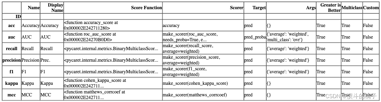
? 设置自定义指标

# 定义一个函数get_metrics，用于获取可用的CV（交叉验证）指标

get_metrics()

在这里插入图片描述

# 导入numpy库
import numpy as np

def custom_metric(y, y_pred):
    tp = np.where((y_pred==1) & (y==1), (100), 0)
    fp = np.where((y_pred==1) & (y==0), -5, 0)
    return np.sum([tp,fp])
# 将自定义指标添加到PyCaret中，指标名称为'custom_metric'，显示名称为'Custom Metric'，计算方法为custom_metric函数
add_metric('custom_metric', 'Custom Metric', custom_metric)

Name                                                  Custom Metric
Display Name                                          Custom Metric
Score Function       <function custom_metric at 0x000002E24B0EA430>
Scorer                                   make_scorer(custom_metric)
Target                                                         pred
Args                                                             {}
Greater is Better                                              True
Multiclass                                                     True
Custom                                                         True
Name: custom_metric, dtype: object

# 现在让我们再次运行compare_models函数

compare_models()  # 调用compare_models函数，用于比较不同模型的性能

在这里插入图片描述

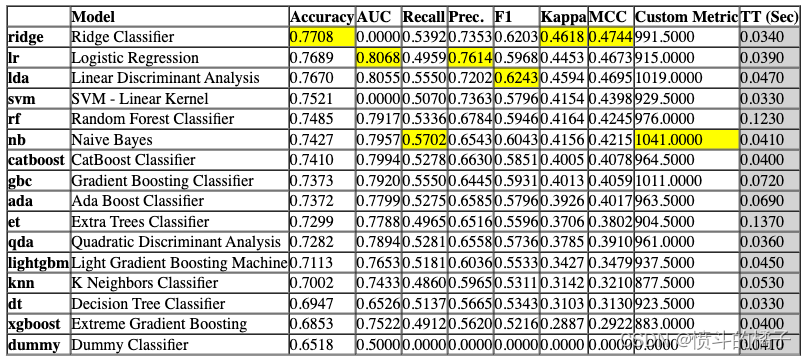
Processing:   0%|          | 0/69 [00:00<?, ?it/s]

在这里插入图片描述

# 移除自定义指标
remove_metric('custom_metric')

? 实验日志记录

PyCaret与许多不同类型的实验记录器集成（默认为’mlflow’）。要在PyCaret中启用实验跟踪，您可以设置log_experiment和experiment_name参数。它将根据定义的记录器自动跟踪所有指标、超参数和工件。

# 使用setup函数对数据进行预处理和建模
# data为数据集，target为目标变量的名称
# log_experiment参数设置为'mlflow'，表示将实验日志记录到mlflow中
# experiment_name参数设置为'diabetes_experiment'，表示实验的名称为diabetes_experiment
s = setup(data, target='Class variable', log_experiment='mlflow', experiment_name='diabetes_experiment')

# 比较模型
# best = compare_models()

# !mlflow ui

默认情况下，PyCaret使用MLFlow记录器，可以使用log_experiment参数进行更改。以下记录器可用：

mlflow
wandb
comet_ml
dagshub

您可能会发现有用的其他与日志记录相关的参数有：

experiment_custom_tags
log_plots
log_data
log_profile

有关更多信息，请查看setup函数的文档字符串。

# help(setup)

? 创建模型

该函数使用交叉验证训练和评估给定估计器的性能。该函数的输出是一个包含每折交叉验证得分的评分网格。可以使用get_metrics函数访问在交叉验证期间评估的指标。可以使用add_metric和remove_metric函数添加或删除自定义指标。可以使用models函数访问所有可用的模型。

# 查看所有可用的模型
models()

在这里插入图片描述

# 使用默认的折叠数（fold=10）来训练逻辑回归模型
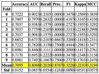
lr = create_model('lr')

在这里插入图片描述

Processing:   0%|          | 0/4 [00:00<?, ?it/s]

功能以上返回训练好的模型对象作为输出。评分表格仅显示而不返回。如果您需要访问评分表格，可以使用pull函数访问数据框。

# 从pull()函数中获取lr_results变量
lr_results = pull()

# 打印lr_results的数据类型
print(type(lr_results))

# 打印lr_results的值

<class 'pandas.core.frame.DataFrame'>

在这里插入图片描述

# 使用逻辑回归算法创建一个模型
# fold=3表示使用3折交叉验证
lr = create_model('lr', fold=3)

在这里插入图片描述

Processing:   0%|          | 0/4 [00:00<?, ?it/s]

# 定义一个函数create_model，用于训练逻辑回归模型，并指定模型参数
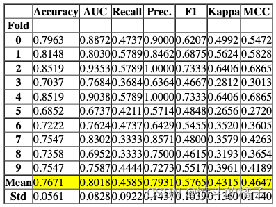
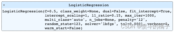
create_model('lr', C = 0.5, l1_ratio = 0.15)

在这里插入图片描述

Processing:   0%|          | 0/4 [00:00<?, ?it/s]

在这里插入图片描述

# 定义函数create_model，用于训练逻辑回归模型，并返回训练得分和交叉验证得分
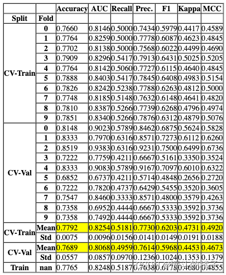
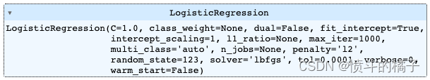
create_model('lr', return_train_score=True)

在这里插入图片描述

Processing:   0%|          | 0/4 [00:00<?, ?it/s]

在这里插入图片描述

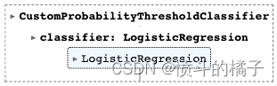
# 创建一个逻辑回归模型，并将分类器的概率阈值设置为0.66
create_model('lr', probability_threshold = 0.66)

在这里插入图片描述

Processing:   0%|          | 0/4 [00:00<?, ?it/s]

在这里插入图片描述

一些在create_model中可能非常有用的其他参数包括：

cross_validation
engine
fit_kwargs
groups

您可以查看函数的文档字符串以获取更多信息。

# help(create_model)

? 调整模型

该函数用于调整模型的超参数。该函数的输出是一个通过交叉验证得到的得分网格。根据优化参数中定义的指标选择最佳模型。可以使用get_metrics函数访问交叉验证期间评估的指标。可以使用add_metric和remove_metric函数添加或删除自定义指标。

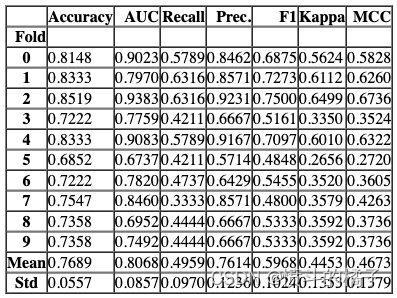
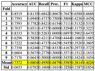
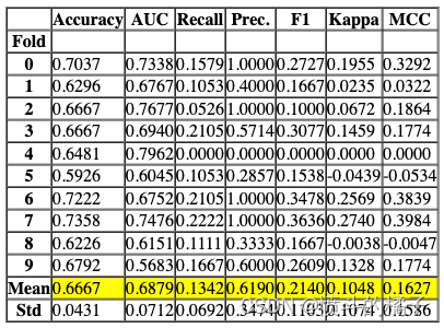
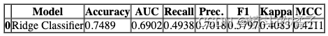
# 使用默认参数创建一个决策树模型
dt = create_model('dt')

在这里插入图片描述

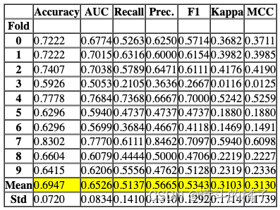
Processing:   0%|          | 0/4 [00:00<?, ?it/s]

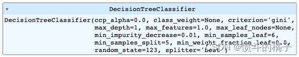
# 调整决策树模型的超参数

# 使用tune_model函数对决策树模型进行超参数调整，并将调整后的模型赋值给tuned_dt变量。
tuned_dt = tune_model(dt)

在这里插入图片描述

Processing:   0%|          | 0/7 [00:00<?, ?it/s]


Fitting 10 folds for each of 10 candidates, totalling 100 fits

可以在 optimize 参数中定义要优化的度量标准（默认为 ‘Accuracy’）。此外，还可以使用 custom_grid 参数传递自定义调整的网格。

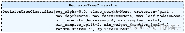
dt

在这里插入图片描述

# 定义调参网格
dt_grid = {'max_depth' : [None, 2, 4, 6, 8, 10, 12]}

# 使用自定义网格和评估指标为F1来调整模型
tuned_dt = tune_model(dt, custom_grid = dt_grid, optimize = 'F1')

在这里插入图片描述

Processing:   0%|          | 0/7 [00:00<?, ?it/s]


Fitting 10 folds for each of 7 candidates, totalling 70 fits

# 使用tune_model函数对决策树模型进行调参，并返回调参后的模型和调参器对象
tuned_dt, tuner = tune_model(dt, return_tuner=True)

# 返回的tuned_dt是经过调参后的决策树模型
# 返回的tuner是用于调参的对象，可以通过该对象访问调参器的属性和方法

在这里插入图片描述

Processing:   0%|          | 0/7 [00:00<?, ?it/s]


Fitting 10 folds for each of 10 candidates, totalling 100 fits

tuned_dt

在这里插入图片描述

# 创建一个调参器对象

# tuner object
tuner

在这里插入图片描述

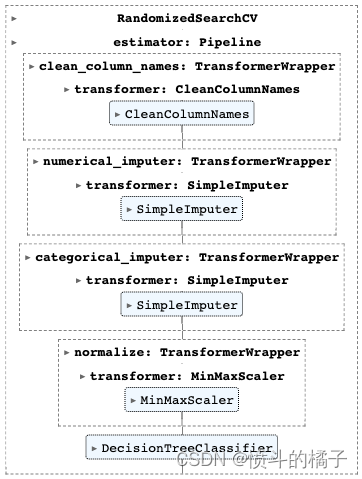
默认的搜索算法是sklearn中的RandomizedSearchCV。可以通过使用search_library和search_algorithm参数来进行更改。

# 使用 Optuna 调整决策树模型（dt）
# 调用 tune_model 函数，传入决策树模型（dt）和搜索库（optuna）
tuned_dt = tune_model(dt, search_library='optuna')

在这里插入图片描述

Processing:   0%|          | 0/7 [00:00<?, ?it/s]


[32m[I 2023-02-16 14:23:58,902][0m Searching the best hyperparameters using 537 samples...[0m
[32m[I 2023-02-16 14:24:07,369][0m Finished hyperparemeter search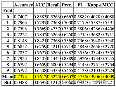![0m

有关所有可用的search_library和search_algorithm的更多详细信息，请查看文档字符串。在tune_model中，您可能会发现一些其他非常有用的参数：

choose_better
n_iter
early_stopping
groups

您可以查看函数的文档字符串以获取更多信息。

# 导入所需的库
from pycaret.classification import *

# 初始化分类模型
clf = setup(data, target='target')

# 调整模型超参数
best_model = tune_model(clf)

# 输出最佳模型的性能指标
print(best_model)

? 集成模型

该函数对给定的估计器进行集成。该函数的输出是一个包含按折叠计算的CV分数的评分网格。可以使用get_metrics函数访问CV期间评估的指标。可以使用add_metric和remove_metric函数添加或删除自定义指标。

# 使用Bagging方法对决策树模型dt进行集成
ensemble_model(dt, method='Bagging')

在这里插入图片描述

Processing:   0%|          | 0/6 [00:00<?, ?it/s]

在这里插入图片描述

# 调用ensemble_model函数，传入参数dt和method
# dt是决策树模型
# method是指定的集成方法，这里是'Boosting'，表示使用Boosting算法进行集成
ensemble_model(dt, method='Boosting')

在这里插入图片描述

Processing:   0%|          | 0/6 [00:00<?, ?it/s]

在这里插入图片描述

一些在ensemble_model中可能非常有用的其他参数有：

choose_better
n_estimators
groups
fit_kwargs
probability_threshold
return_train_score

您可以查看函数的文档字符串以获取更多信息。

# 导入ensemble_model模块
import ensemble_model

# 调用ensemble_model模块中的函数
ensemble_model.function()

? 混合模型

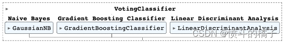
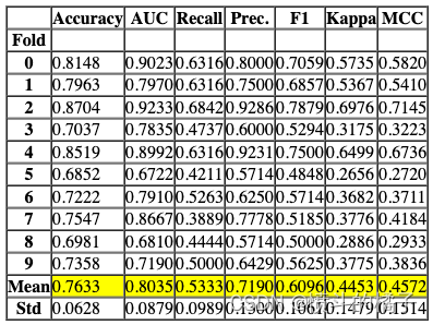
该函数用于训练一个软投票/多数规则分类器，该分类器选择在estimator_list参数中传递的模型。该函数的输出是一个包含交叉验证得分的评分网格。可以使用get_metrics函数访问在交叉验证期间评估的指标。可以使用add_metric和remove_metric函数添加或删除自定义指标。

# 定义一个变量best_recall_models_top3，用于存储基于召回率的前三个模型的信息
best_recall_models_top3

[GaussianNB(priors=None, var_smoothing=1e-09),
 GradientBoostingClassifier(ccp_alpha=0.0, criterion='friedman_mse', init=None,
                            learning_rate=0.1, loss='log_loss', max_depth=3,
                            max_features=None, max_leaf_nodes=None,
                            min_impurity_decrease=0.0, min_samples_leaf=1,
                            min_samples_split=2, min_weight_fraction_leaf=0.0,
                            n_estimators=100, n_iter_no_change=None,
                            random_state=123, subsample=1.0, tol=0.0001,
                            validation_fraction=0.1, verbose=0,
                            warm_start=False),
 LinearDiscriminantAnalysis(covariance_estimator=None, n_components=None,
                            priors=None, shrinkage=None, solver='svd',
                            store_covariance=False, tol=0.0001)]

# blend_models函数用于将最佳召回率的前三个模型进行融合

# 参数best_recall_models_top3是一个包含最佳召回率的前三个模型的列表

# 在这个函数中，我们将使用某种方法将这三个模型进行融合，以期望得到更好的结果

# 返回值是融合后的模型
blend_models(best_recall_models_top3)

在这里插入图片描述

Processing:   0%|          | 0/6 [00:00<?, ?it/s]

在这里插入图片描述

一些在blend_models中可能非常有用的其他参数包括：

choose_better
method
weights
fit_kwargs
probability_threshold
return_train_score

您可以查看函数的文档字符串以获取更多信息。

# help(blend_models)

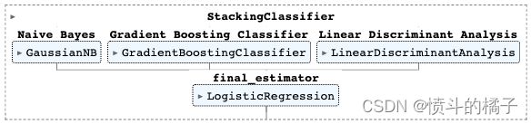
? 堆叠模型

该函数在estimator_list参数中传递的选择估计器上训练一个元模型。该函数的输出是一个包含每个折叠的CV分数的评分网格。可以使用get_metrics函数访问CV期间评估的指标。可以使用add_metric和remove_metric函数添加或删除自定义指标。

# 将模型堆叠起来

# 参数：
# best_recall_models_top3: 一个包含了最佳召回率的前三个模型的列表

stack_models(best_recall_models_top3)

在这里插入图片描述

Processing:   0%|          | 0/6 [00:00<?, ?it/s]

在这里插入图片描述

任务：请翻译以下markdown为中文，请保留markdown的格式，并输出翻译结果。

语料:
一些在stack_models中可能非常有用的其他参数包括：

choose_better
meta_model
method
restack
probability_threshold
return_train_score

您可以查看函数的文档字符串以获取更多信息。

# help(stack_models)

? 绘制模型

该函数用于分析训练好的模型在留置集上的性能。在某些情况下，可能需要重新训练模型。

# 调用函数绘制分类报告图表
plot_model(best, plot = 'class_report')

在这里插入图片描述

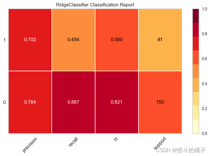
# 绘制模型评估报告的图表
# best: 最佳模型
# plot = 'class_report': 绘制分类报告
# scale = 2: 控制图表的缩放比例为2
plot_model(best, plot='class_report', scale=2)

在这里插入图片描述

# 保存分类报告的绘图
plot_model(best, plot = 'class_report', save=True)

'Class Report.png'

一些在plot_model中可能非常有用的其他参数包括：

fit_kwargs
plot_kwargs
groups
display_format

您可以查看函数的文档字符串以获取更多信息。

# help(plot_model)

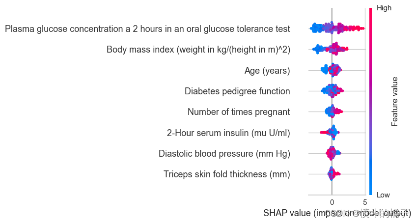
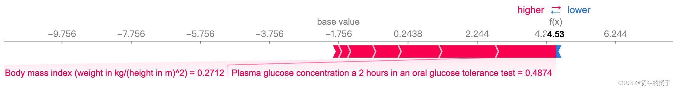
? 解释模型

该函数分析训练模型生成的预测结果。该函数中的大多数图表是基于SHAP（Shapley Additive exPlanations）实现的。有关更多信息，请参见https://shap.readthedocs.io/en/latest/

# 使用'lightgbm'算法创建一个分类模型
lightgbm = create_model('lightgbm')

在这里插入图片描述

Processing:   0%|          | 0/4 [00:00<?, ?it/s]

# 使用interpret_model函数对模型进行解释
# 参数lightgbm表示使用的模型为lightgbm模型
# 参数plot表示是否绘制模型的摘要图，默认为True
interpret_model(lightgbm, plot='summary')

在这里插入图片描述

# 使用lightgbm模型解释测试集观察值1的原因图
interpret_model(lightgbm, plot='reason', observation=1)

在这里插入图片描述

一些在interpret_model中可能非常有用的其他参数有：

plot
feature
use_train_data
X_new_sample
y_new_sample
save

您可以查看函数的文档字符串以获取更多信息。

# help(interpret_model)

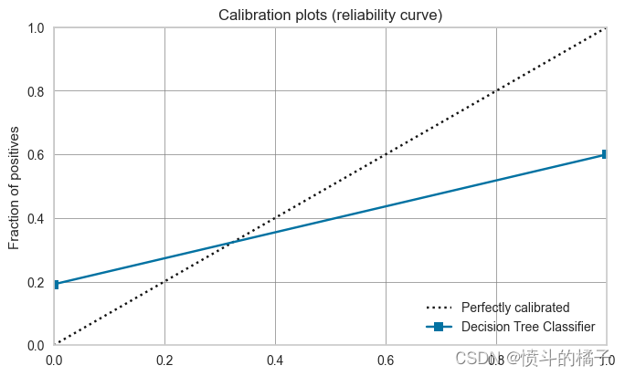
? 校准模型

该函数使用保序回归或逻辑回归来校准给定模型的概率。该函数的输出是一个带有交叉验证得分的评分网格。可以使用get_metrics函数访问CV期间评估的指标。可以使用add_metric和remove_metric函数添加或删除自定义指标。

# 绘制决策树的校准图
# 参数plot='calibration'表示绘制校准图
plot_model(dt, plot='calibration')

在这里插入图片描述

# 设置默认的时间间隔（dt）校准
calibrated_dt = calibrate_model(dt)

在这里插入图片描述

Processing:   0%|          | 0/6 [00:00<?, ?it/s]

# 使用plot_model函数绘制校准后的决策树模型的校准曲线图
# 参数calibrated_dt表示校准后的决策树模型
# 参数plot='calibration'表示绘制校准曲线图
plot_model(calibrated_dt, plot='calibration')

在这里插入图片描述

一些在calibrate_model中可能非常有用的其他参数包括：

calibrate_fold
fit_kwargs
method
return_train_score
groups

您可以查看函数的文档字符串以获取更多信息。

# help(calibrate_model)

? 获取排行榜

该函数返回当前设置中训练的所有模型的排行榜。

# 获取排行榜
lb = get_leaderboard()

Processing:   0%|          | 0/76 [00:00<?, ?it/s]

在这里插入图片描述

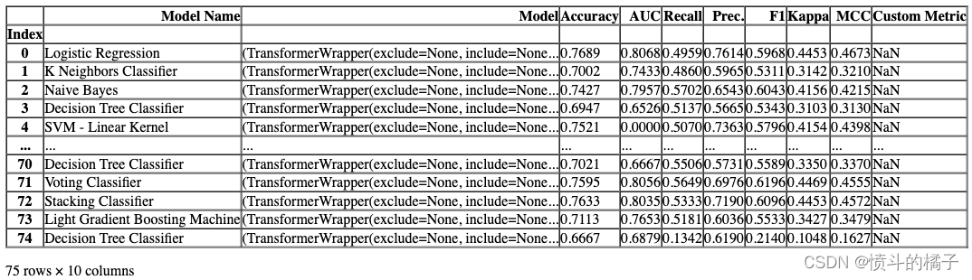
# 根据F1值选择最佳模型
# 使用sort_values方法对数据框lb按照F1列进行降序排序
# 使用['Model']索引选择'Model'列
# 使用iloc[0]选择排序后的第一个模型作为最佳模型
lb.sort_values(by='F1', ascending=False)['Model'].iloc[0]

在这里插入图片描述

任务：请翻译以下markdown为中文，请保留markdown的格式，并输出翻译结果。

语料:
一些你可能会在get_leaderboard中发现非常有用的其他参数有：

finalize_models
fit_kwargs
model_only
groups

你可以查看函数的文档字符串以获取更多信息。

# help(get_leaderboard)

? AutoML

该函数根据优化参数返回当前设置中所有训练模型中的最佳模型。可以使用get_metrics函数访问评估的指标。

automl()

在这里插入图片描述

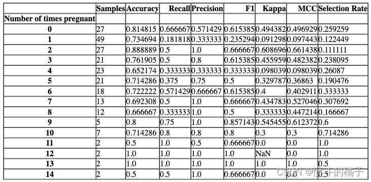
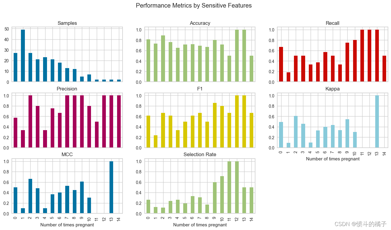
? 检查公平性

有许多方法可以概念化公平性。check_fairness函数遵循被称为群体公平性的方法，它询问：哪些个体群体有可能遭受伤害。check_fairness提供了不同群体（也称为子群体）之间的公平性相关指标。

# 检查公平性
# best: 模型的最佳参数
# sensitive_features: 敏感特征，用于评估模型的公平性

check_fairness(best, sensitive_features = ['Number of times pregnant'])

在这里插入图片描述

? 仪表盘

仪表盘功能用于为训练模型生成交互式仪表盘。该仪表盘是使用ExplainerDashboard实现的。更多信息请查看Explainer Dashboard.

# 定义一个名为dashboard的函数
# 参数dt：表示数据表格
# 参数display_format：表示显示格式，默认为'inline'，即内联显示

# 函数功能：用于创建一个仪表盘，用于展示数据表格dt的内容

dashboard(dt, display_format ='inline')

Note: model_output=='probability', so assuming that raw shap output of DecisionTreeClassifier is in probability space...
Generating self.shap_explainer = shap.TreeExplainer(model)
Building ExplainerDashboard..
The explainer object has no decision_trees property. so setting decision_trees=False...
Warning: calculating shap interaction values can be slow! Pass shap_interaction=False to remove interactions tab.
Generating layout...
Calculating shap values...
Calculating prediction probabilities...
Calculating metrics...
Calculating confusion matrices...
Calculating classification_dfs...
Calculating roc auc curves...
Calculating pr auc curves...
Calculating liftcurve_dfs...
Calculating shap interaction values... (this may take a while)
Reminder: TreeShap computational complexity is O(TLD^2), where T is the number of trees, L is the maximum number of leaves in any tree and D the maximal depth of any tree. So reducing these will speed up the calculation.
Calculating dependencies...
Calculating permutation importances (if slow, try setting n_jobs parameter)...
Calculating predictions...
Calculating pred_percentiles...
Reminder: you can store the explainer (including calculated dependencies) with explainer.dump('explainer.joblib') and reload with e.g. ClassifierExplainer.from_file('explainer.joblib')
Registering callbacks...
Starting ExplainerDashboard inline (terminate it with ExplainerDashboard.terminate(8050))

?创建应用程序

此函数创建一个用于推理的基本 gradio 应用程序。

# 创建一个Gradio应用程序

# 参数：
# - best: 一个变量，表示最佳模型

create_app(best)  # 调用create_app函数，并传入best作为参数，创建一个Gradio应用程序

Running on local URL:  http://127.0.0.1:7860

To create a public link, set `share=True` in `launch()`.

? 创建API

该函数接受一个输入模型，并创建一个用于推理的POST API。

# 创建API
# 参数：
# - best: 最佳模型
# - api_name: API的名称，默认为'my_first_api'
create_api(best, api_name='my_first_api')

API successfully created. This function only creates a POST API, it doesn't run it automatically. To run your API, please run this command --> !python my_first_api.py

# !python my_first_api.py

# %load my_first_api.py

? 创建Docker

此函数用于创建Dockerfile和requirements.txt，以便将API端点投入生产。

# 定义一个函数create_docker，用于创建一个名为'my_first_api'的Docker容器
create_docker('my_first_api')

Writing requirements.txt
Writing Dockerfile
Dockerfile and requirements.txt successfully created.
    To build image you have to run --> !docker image build -f "Dockerfile" -t IMAGE_NAME:IMAGE_TAG .

# 检查使用这个神奇命令创建的DockerFile文件
# %load DockerFile

# 检查使用魔法命令创建的requirements.txt文件
# %load requirements.txt

? 完善模型

该函数在整个数据集上训练给定的模型，包括留出集。

# 将模型进行最终的优化
final_best = finalize_model(best)

final_best

在这里插入图片描述

? 转换模型

该函数将训练好的机器学习模型的决策函数转换为不同的编程语言，如Python、C、Java、Go、C#等。如果您想要将模型部署到无法安装正常的Python环境来支持模型推理的环境中，这将非常有用。

# 将学习到的函数转换为Java代码
# 调用convert_model函数，将学习到的函数转换为Java代码，并指定目标语言为Java
# best是学习到的函数
# language参数指定目标语言为Java
# 打印转换后的Java代码
print(convert_model(best, language = 'java'))

public class Model {
    public static double score(double[] input) {
        return -2.4222329408494767 + input[0] * 0.5943492729771869 + input[1] * 2.3273354603187455 + input[2] * -0.41637843900032867 + input[3] * 0.10259178891131746 + input[4] * -0.3134524281639536 + input[5] * 1.4903417391961826 + input[6] * 0.5019685413792472 + input[7] * 0.12389520576261319;
    }
}

? 部署模型

此函数在云上部署整个机器学习流程。

AWS: 在AWS S3上部署模型时，必须使用命令行界面配置环境变量。要配置AWS环境变量，请在终端中输入aws configure命令。需要以下信息，可以使用您的Amazon控制台帐户的身份和访问管理（IAM）门户生成：

AWS访问密钥ID
AWS秘密密钥访问
默认区域名称（可以在AWS控制台的全局设置下看到）
默认输出格式（必须留空）

GCP: 要在Google Cloud Platform（‘gcp’）上部署模型，必须使用命令行或GCP控制台创建项目。创建项目后，您必须创建一个服务帐户，并将服务帐户密钥下载为JSON文件，以在本地环境中设置环境变量。了解更多信息：https://cloud.google.com/docs/authentication/production

Azure: 要在Microsoft Azure（‘azure’）上部署模型，必须在本地环境中设置用于连接字符串的环境变量。转到Azure门户上的存储帐户设置以访问所需的连接字符串。
AZURE_STORAGE_CONNECTION_STRING（作为环境变量必需）
了解更多信息：https://docs.microsoft.com/en-us/azure/storage/blobs/storage-quickstart-blobs-python?toc=%2Fpython%2Fazure%2FTOC.json

# 部署模型到AWS S3
# 调用函数来部署模型
deploy_model(best, model_name='my_first_platform_on_aws', platform='aws', authentication={'bucket': 'pycaret-test'})

# 从AWS S3加载模型
# 从AWS S3加载模型的代码被注释掉了，可能是因为没有提供完整的代码或者没有正确的身份验证信息。

# 加载模型
# loaded_from_aws = load_model(model_name='my_first_platform_on_aws', platform='aws',
#                              authentication={'bucket': 'pycaret-test'})

# loaded_from_aws

? 保存/加载模型

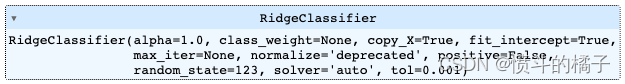
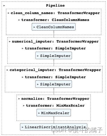
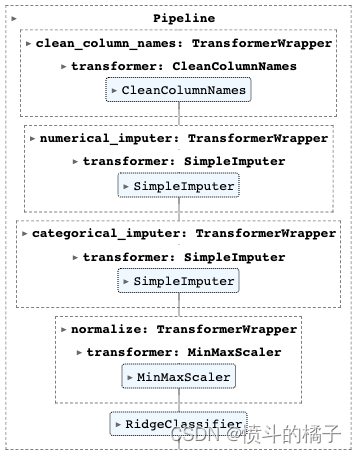
这个函数将转换流水线和训练好的模型对象保存到当前工作目录中，以pickle文件的形式供以后使用。

# 保存模型
# 使用save_model函数将最佳模型保存为'my_first_model'文件
save_model(best, 'my_first_model')

Transformation Pipeline and Model Successfully Saved





(Pipeline(memory=FastMemory(location=C:\Users\owner\AppData\Local\Temp\joblib),
          steps=[('clean_column_names',
                  TransformerWrapper(exclude=None, include=None,
                                     transformer=CleanColumnNames(match='[\\]\\[\\,\\{\\}\\"\\:]+'))),
                 ('numerical_imputer',
                  TransformerWrapper(exclude=None,
                                     include=['Number of times pregnant',
                                              'Plasma glucose concentration a 2 '
                                              'hours in an oral glu...
                                                               verbose='deprecated'))),
                 ('normalize',
                  TransformerWrapper(exclude=None, include=None,
                                     transformer=MinMaxScaler(clip=False,
                                                              copy=True,
                                                              feature_range=(0,
                                                                             1)))),
                 ('trained_model',
                  RidgeClassifier(alpha=1.0, class_weight=None, copy_X=True,
                                  fit_intercept=True, max_iter=None,
                                  normalize='deprecated', positive=False,
                                  random_state=123, solver='auto', tol=0.001))],
          verbose=False),
 'my_first_model.pkl')

# 加载模型
loaded_from_disk = load_model('my_first_model')
loaded_from_disk
# 从磁盘中加载模型文件 'my_first_model'，并将其赋值给变量 loaded_from_disk

Transformation Pipeline and Model Successfully Loaded

在这里插入图片描述

? 保存/加载实验

该函数将实验中的所有变量保存到磁盘上，以便以后恢复而无需重新运行设置函数。

# 保存实验
save_experiment('my_experiment')

# 从磁盘加载实验
exp_from_disk = load_experiment('my_experiment', data=data)

在这里插入图片描述

本代码链接

https://download.csdn.net/download/wjjc1017/88646143

文章来源:https://blog.csdn.net/wjjc1017/article/details/135101062
本文来自互联网用户投稿，该文观点仅代表作者本人，不代表本站立场。本站仅提供信息存储空间服务，不拥有所有权，不承担相关法律责任。如若内容造成侵权/违法违规/事实不符，请联系我的编程经验分享网邮箱：veading@qq.com进行投诉反馈，一经查实，立即删除！