Discrete Time Signals and Systems
Discrete Time Signals and Systems
文章目录
- Discrete Time Signals and Systems
- Signal classification
- basic signal
- Operation on signal
- System of discrete signal
- Fourier Series
- Continuous time Fourier transform (CTFT)
- Fourier transform of Periodic signal
- Discrete time fouriew series (DTFT)
- Discrete Fourier Transform(DFT)
- z-transformation
Signal classification
- Periodic and non-periodic
- Odd and even signals
- energy signal and power signal
basic signal
- Impulse function
- unit step function
- Ramp function
Operation on signal
?
Periodic and Aperiodic Discrete-Time Sinusoids
x
(
n
)
=
A
c
o
s
[
2
π
f
0
n
]
=
x
(
n
+
N
)
=
A
c
o
s
[
2
π
f
0
(
n
+
N
)
]
=
A
c
o
s
[
2
π
f
0
n
+
2
π
f
0
N
]
x(n)=Acos[2 \pi f_0 n]=x(n+N)=Acos[2 \pi f_0 (n+N)]=Acos[2 \pi f_0 n+2 \pi f_0 N]
x(n)=Acos[2πf0?n]=x(n+N)=Acos[2πf0?(n+N)]=Acos[2πf0?n+2πf0?N]
2
π
f
0
N
=
2
π
k
2\pi f_0 N =2 \pi k
2πf0?N=2πk just
f
0
=
k
N
f_0 = \frac{k}{N}
f0?=Nk?
n is integer: Periodic
n is not integer: Aperiodic
Periodic judgment of composite signals
-
Find N for each signal
if N 1 N 2 = r a t i o n a l ? n u m b e r \frac{N_1}{N_2} = rational \ number N2?N1??=rational?number it is Periodic
-
Find the lowest common multiple($ LCM(N_1,N_2)$)
Periodic is L C M ( N 1 , N 2 ) LCM(N_1,N_2) LCM(N1?,N2?)
Odd and even signals
odd: x 0 ( t ) = 1 2 [ x ( t ) ? x ( ? t ) ] x_0(t)=\frac{1}{2}[x(t)-x(-t)] x0?(t)=21?[x(t)?x(?t)]
even: x e ( t ) = 1 2 [ x ( t ) + x ( ? t ) ] x_e(t) = \frac{1}{2}[x(t)+x(-t)] xe?(t)=21?[x(t)+x(?t)]
x ( t ) = x 0 ( t ) + x e ( t ) x(t) = x_0(t) + x_e(t) x(t)=x0?(t)+xe?(t)
energy signal and power signal
energy: E = ∑ n = ? ∞ ∞ ∣ x [ n ] ∣ 2 E=\sum_{n=-\infty}^{\infty}|x[n]|^2 E=∑n=?∞∞?∣x[n]∣2
power:
Periodic: P ∞ = lim ? N → ∞ 1 2 N + 1 ∑ n = ? ∞ + ∞ ∣ x [ n ] ∣ 2 P_\infty=\lim_{N\to\infty}\frac1{2N+1}\sum_{n=-\infty}^{+\infty}|x[n]|^2 P∞?=limN→∞?2N+11?∑n=?∞+∞?∣x[n]∣2
Aperiodic: P x = 1 N ∑ n = 0 N ? 1 ∣ x [ n ] ∣ 2 P_x=\frac1{N}\sum_{n=0}^{N-1}|x[n]|^2 Px?=N1?∑n=0N?1?∣x[n]∣2
energy signal:energy is finite,power is zero
power signal:energy is infinite,power is finite
?
find the energy and power for
- Impulse function
- unit step function
- Ramp function
?
- Time Shifting(left is +;right is -)
- Time-scale
- Time Reversal
?
System of discrete signal
-
Linear systems and nonlinear systems
-
Causal and Acausal Systems
-
Time-varying and time-invariant systems
-
static system and dynamic system
-
Stable and unstable systems
-
convolution
-
convolution sum
-
circular convolution
-
Stability of linear time-invariant systems
Linear systems and nonlinear systems
- Linear systems satisfy uniformity and superposition
- A system that satisfies uniformity and superposition is a linear system
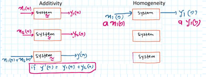
Must have: x ( n ) = y ( n ) = 0 x(n) = y(n) = 0 x(n)=y(n)=0
Four steps to solve problems:
- x1 to y1 = F(x1)
- x2 to y2 = F(x2)
- y3 = ay1 + by2
- F(ax1 +bx2) = y4
if y4 = y3 ,the system is linear
?
Causal and non-causal Systems
casual system: The output depends only on present and past signals
Acausal Systems:The output depends on at least one future input
eg:Y(n) = x(-n) is non-casual (at n = -1)
even and odd is non-casual
ps: anti-casual system: output only upon “only future input” for all time
?
Time-varying and time-invariant systems
Time-varying system(TVS):
y(n) = F[x(n)] = x(n)cos(2 w π w \pi wπn)
y(n,k) = F[x(n-k)] = x(n-k)cos(2 w π w \pi wπn)
y(n-k) ≠ \ne = y(n,k)
y(n) to y(n,k):only change n for x(n)
time-invariant systems :
y(n,k) = y(n-k)
eg:y(n-k) = sin (x(n-k))
y change n for all n
?
static system and dynamic system
static system (memory-less system):
output only depends on now input for all time
dynamic system:
output depends on past and/or future inputs
?
Stable and unstable systems
Stable system: BIBO
bounded input to bounded output
unstable systems:
bounded input to unbounded output
eg: y ( n ) = y 2 ( n ? 1 ) + 2 δ ( n ) y(n)=y^2(n-1)+2\delta (n) y(n)=y2(n?1)+2δ(n)
?
convolution
- time-invariant systems
y ( n ) = ∑ k = ? ∞ ∞ x ( k ) h ( n ? k ) y(n)=\sum_{k=-\infty}^{\infty}x(k)h(n-k) y(n)=∑k=?∞∞?x(k)h(n?k)
y ( n ) = x ( n ) ? h ( n ) y(n)=x(n)*h(n) y(n)=x(n)?h(n)
- time reversal
- shifting of h(-k) to h(n-k)
- multiply x(k)h(n-k)
- Sum
- linear convolution
- circular convolution
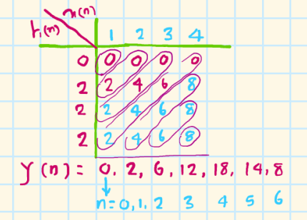
matrix method:
x(n) = {1,2,3,4} h(n)={0,2,2,2}
length of x(n):4 samples;k
length of h(n):4 samples;m
length of y(n): = k + m - 1 = 4 + 4 - 1 = 7 samples
?
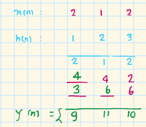
circular convolution
x(n) = {2,1,2} h(n) = {1,2,3}
y ( n ) = ∑ k = ? ∞ ∞ x ( k ) h ( n ? k ) y(n)=\sum_{k=-\infty}^{\infty}x(k)h(n-k) y(n)=∑k=?∞∞?x(k)h(n?k)
?
Stability of linear time-invariant systems
S = ∑ k = ? ∞ ∞ ∣ h ( n ) ∣ < ∞ S=\sum_{k=-\infty}^{\infty}|h(n)| < \infty S=∑k=?∞∞?∣h(n)∣<∞
it is stability
eg: h ( n ) = ( 0.8 ) n u ( n + 2 ) h(n) = (0.8)^n u(n+2) h(n)=(0.8)nu(n+2)
?
Fourier Series
- Fourier Series basic concepts
- Discrete time fouriew series (DTFS)
Fourier Series basic concepts
Condition for existence of Fourier Series
- Finite Number of maxima and minima over the time period
- Finite number of discontinuities over the time period T
- Signal should be absolutely integrable over the range of time period T
period function:
f ( x ) = a 0 + ∑ n = 1 ∞ ( a n c o s ( n w 0 t ) + b n s i n ( n w 0 t ) f(x)=a_0+\sum_{n=1}^\infty(a_ncos(nw_0t)+b_n sin(nw_0t) f(x)=a0?+∑n=1∞?(an?cos(nw0?t)+bn?sin(nw0?t)
a 0 = 1 T 1 ∫ 0 T 1 f ( t ) d t a_{0}=\frac{1}{T_{1}}\int_{0}^{T_1}f(t)dt a0?=T1?1?∫0T1??f(t)dt
a n = 2 T 1 ∫ 0 T 1 f ( t ) cos ? n w 1 t d t a_{n}=\frac{2}{T_{1}}\int_{0}^{T_{1}}f(t)\cos nw_1tdt an?=T1?2?∫0T1??f(t)cosnw1?tdt
b n = 2 T 1 ∫ 0 T 1 f ( t ) sin ? n w 1 t d t b_{n}=\frac{2}{T_{1}}\int_{0}^{T_{1}}f(t)\sin nw_1tdt bn?=T1?2?∫0T1??f(t)sinnw1?tdt
eg: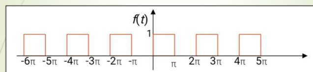
?
Discrete time fouriew series (DTFS)
x n = ∑ k = 0 N ? 1 c ( k ) e J k 2 π N n x_n=\sum_{k=0}^{N-1}c(k)e^{Jk\frac{2\pi }{N}n} xn?=∑k=0N?1?c(k)eJkN2π?n
c ( k ) = 1 N ∑ n = 0 N ? 1 x ( n ) e ? J k 2 π N n c(k)=\frac{1}{N}\sum_{n=0}^{N-1}x(n)e^{-Jk\frac{2\pi}{N}n} c(k)=N1?∑n=0N?1?x(n)e?JkN2π?n
?
CTFS
x ( w ) = ∫ ? ∞ + ∞ x ( t ) e ? J w t d t x(w)=\int_{-\infty}^{+\infty}x(t)e^{-Jwt}dt x(w)=∫?∞+∞?x(t)e?Jwtdt
Inverse transformation: x ( t ) = 1 2 π ∫ ? ∞ + ∞ x ( w ) e j w t d w x(t)=\frac{1}{2\pi}\int_{-\infty}^{+\infty}x(w)e^{jwt}dw x(t)=2π1?∫?∞+∞?x(w)ejwtdw
?
Continuous time Fourier transform (CTFT)
- basic concept
- fourier fransform
- magnitude specturm
- phase spectrum
properties of CTFT
- linearity
- time shifting
- frequency shifting
- time scaling
- time differenciation
- frequency differenciation
- convolution
Parseval’s Theorem
-
Any signal is built up addition of elementary signals which are at different frequencies.
-
CTFT is used to transform the signal from time domain to frequency domain.
-
With the help of CTFT,plot the amplitude and phase spectrum.
-
CTFT can be efxpressed as:
x ( w ) = ∫ ? ∞ + ∞ x ( t ) e ? J w t d t x(w)=\int_{-\infty}^{+\infty}x(t)e^{-Jwt}dt x(w)=∫?∞+∞?x(t)e?Jwtdt
Inverse transformation: x ( t ) = 1 2 π ∫ ? ∞ + ∞ x ( w ) e j w t d w x(t)=\frac{1}{2\pi}\int_{-\infty}^{+\infty}x(w)e^{jwt}dw x(t)=2π1?∫?∞+∞?x(w)ejwtdw
?
Dirichlet’s conditions
- f(t) should be absolutely integrable.
- f(t) should have a finite number of maxima and minima over any finite interval.
- f(t) should have finite number of discontinues over any finite interval
These conditions are sufficient but not necessary Condition.
If the conditions are not met, there is not necessarily no Fourier transform.
?
lecture(77)
- fourier fransform
- magnitude specturm
- phase spectrum
?
lecture(78)
Inverse transformation for function
important
?
properties of CTFT
linearity
F [ f ( t ) ] = F ( ω ) , F [ g ( t ) ] = G ( ω ) \mathscr{F}[f(t)]=F(\omega),\quad\mathscr{F}[g(t)]=G(\omega) F[f(t)]=F(ω),F[g(t)]=G(ω)
F [ α f ( t ) + β g ( t ) ] = α F ( ω ) + β G ( ω ) F ? 1 [ α F ( ω ) + β G ( ω ) ] = α f ( t ) + β g ( t ) \begin{aligned}\mathscr{F}[\alpha f(t)+\beta g(t)]&=\alpha F(\omega)+\beta G(\omega)\\\mathscr{F}^{-1}[\alpha F(\omega)+\beta G(\omega)]&=\alpha f(t)+\beta g(t)\end{aligned} F[αf(t)+βg(t)]F?1[αF(ω)+βG(ω)]?=αF(ω)+βG(ω)=αf(t)+βg(t)?
time shifting
F [ f ( t ) ] = F ( ω ) \mathcal{F}[f(t)]=F(\omega) F[f(t)]=F(ω)
F [ f ( t ? t 0 ) ] = e ? j ω t 0 F ( ω ) F ? 1 [ F ( ω ? ω 0 ) ] = e j ω 0 t f ( t ) \begin{aligned}\mathscr{F}[f(t-t_0)]&=e^{-j\omega t_0}F(\omega)\\\mathscr{F}^{-1}[F(\omega-\omega_0)]&=e^{j\omega_0t}f(t)\end{aligned} F[f(t?t0?)]F?1[F(ω?ω0?)]?=e?jωt0?F(ω)=ejω0?tf(t)?
time scaling
F [ f ( t ) ] = F ( ω ) \mathcal{F}[f(t)]=F(\omega) F[f(t)]=F(ω)
F [ f ( a t ) ] = 1 ∣ a ∣ F ( ω a ) \mathscr{F}[f(at)]=\frac{1}{|a|}F\left(\frac{\omega}{a}\right) F[f(at)]=∣a∣1?F(aω?)
frequency shifting
F [ f ( t ) ] = F ( ω ) \mathcal{F}[f(t)]=F(\omega) F[f(t)]=F(ω)
F [ f ( t ) e j w 0 t ] = F ( ω ? ω 0 ) F ? 1 [ f ( t ) e ? j w 0 t ] = F ( ω + ω 0 ) \begin{aligned}\mathscr{F}[f(t)e^{jw_0t}]&=F(\omega - \omega_0)\\\mathscr{F}^{-1}[f(t)e^{-jw_0t}]&=F(\omega + \omega_0)\end{aligned} F[f(t)ejw0?t]F?1[f(t)e?jw0?t]?=F(ω?ω0?)=F(ω+ω0?)?
time differenciation
F [ f ( t ) ] = F ( ω ) \mathcal{F}[f(t)]=F(\omega) F[f(t)]=F(ω)
F [ d n f ( t ) d t n ] = ( j ω ) n F ( ω ) F ? 1 [ d n F ( ω ) d ω n ] = ( ? j t ) n f ( t ) \begin{gathered} \mathscr{F}\left[\frac{d^{n}f(t)}{dt^{n}}\right]=(j\omega)^{n}F(\omega) \\ \mathscr{F}^{-1}\left[\frac{d^{n}F(\omega)}{d\omega^{n}}\right]=(-jt)^{n}f(t) \end{gathered} F[dtndnf(t)?]=(jω)nF(ω)F?1[dωndnF(ω)?]=(?jt)nf(t)?
frequency differenciation
F [ f ( t ) ] = F ( ω ) \mathcal{F}[f(t)]=F(\omega) F[f(t)]=F(ω)
F [ ( ? j t ) n f ( t ) ] = d n F ( w ) d w n \mathscr{F} [(-jt)^{n}f(t)]= \frac{d^{n}F(w)}{dw^{n}} F[(?jt)nf(t)]=dwndnF(w)?
F [ t f ( t ) ] = j d F ( w ) d w \mathscr{F} [tf(t)]= j\frac{dF(w)}{dw} F[tf(t)]=jdwdF(w)?
convolution
F [ f ( t ) ] = F ( ω ) , F [ g ( t ) ] = G ( ω ) \mathscr{F}[f(t)]=F(\omega),\quad\mathscr{F}[g(t)]=G(\omega) F[f(t)]=F(ω),F[g(t)]=G(ω)
F [ f 1 ( t ) ? f 2 ( t ) ] = F 1 ( ω ) ? F 2 ( ω ) \mathscr{F}[f_1(t) *f_2(t)]=F_1(\omega)·F_2(\omega) F[f1?(t)?f2?(t)]=F1?(ω)?F2?(ω)
F [ f 1 ( t ) ? f 2 ( t ) ] = 1 2 π F 1 ( ω ) ? F 2 ( ω ) \mathscr{F}[f_1(t) ·f_2(t)]=\frac{1}{2\pi}F_1(\omega)*F_2(\omega) F[f1?(t)?f2?(t)]=2π1?F1?(ω)?F2?(ω)
?
Parseval’s Theorem
if x(t) CTFT to x ( w ) x(w) x(w) or x ( f ) x(f) x(f)
E = ∫ ? ∞ ∞ ∣ x ( t ) ∣ 2 d t = ∫ ? ∞ ∞ ∣ x ( f ) ∣ 2 d f E=\int_{-\infty}^{\infty}|x(t)|^{2}dt=\int_{-\infty}^{\infty}|x(f)|^{2}df E=∫?∞∞?∣x(t)∣2dt=∫?∞∞?∣x(f)∣2df
?
Fourier transform of Periodic signal
- spectrum of e j ω 0 t e^{j\omega_0t } ejω0?t and e ? j ω 0 t e^{- j\omega_0t } e?jω0?t
- spectrum of s i n w t sinwt sinwt and c o s w t coswt coswt
- Spectrum of a general periodic signal
spectrum of e j ω 0 t e^{j\omega_0t } ejω0?t and e ? j ω 0 t e^{- j\omega_0t } e?jω0?t
F [ e j ω 0 t ] = 2 π δ ( ω ? ω 0 ) F [ e ? j ω 0 t ] = 2 π δ ( ω + ω 0 ) \begin{aligned}\mathscr{F}[e^{j\omega_0t}]&=2\pi\delta(\omega-\omega_0)\\\mathscr{F}[e^{-j\omega_0t}]&=2\pi\delta(\omega+\omega_0)\end{aligned} F[ejω0?t]F[e?jω0?t]?=2πδ(ω?ω0?)=2πδ(ω+ω0?)?
?
spectrum of s i n w 0 t sinw_0t sinw0?t and c o s w 0 t cosw_0t cosw0?t
F [ cos ? ( ω 0 t ) ] = F [ e j ω 0 t + e ? j ω 0 t 2 ] = π [ δ ( ω ? ω 0 ) + δ ( ω + ω 0 ) ] F [ sin ? ( ω 0 t ) ] = F [ e j ω 0 t ? e ? j ω 0 t 2 j ] = j π [ δ ( ω + ω 0 ) ? δ ( ω ? ω 0 ) ] \begin{gathered} \mathscr{F}[\cos(\omega_{0}t)]=\mathscr{F}[\frac{e^{j\omega_{0}t}+e^{-j\omega_{0}t}}{2}]=\pi[\delta(\omega-\omega_{0})+\delta(\omega+\omega_{0})] \\ \mathscr{F}[\sin(\omega_{0}t)]=\mathscr{F}[\frac{e^{j\omega_{0}t}-e^{-j\omega_{0}t}}{2j}]=j\pi[\delta(\omega+\omega_{0})-\delta(\omega-\omega_{0})] \end{gathered} F[cos(ω0?t)]=F[2ejω0?t+e?jω0?t?]=π[δ(ω?ω0?)+δ(ω+ω0?)]F[sin(ω0?t)]=F[2jejω0?t?e?jω0?t?]=jπ[δ(ω+ω0?)?δ(ω?ω0?)]?
?
Spectrum of a general periodic signal
f ( t ) = ∑ n = ? ∞ ∞ F ( n w 0 ) e j n w 0 t f(t)=\sum_{n=-\infty}^{\infty}F(nw_0)e^{jnw_0 t} f(t)=∑n=?∞∞?F(nw0?)ejnw0?t
F ( w ) = F [ f ( t ) ] = 2 π ∑ n = ? ∞ ∞ F ( n w 0 ) δ ( ω ? n ω 0 ) F(w) = \mathscr{F}[f(t)] = 2\pi \sum_{n=-\infty}^{\infty}F(nw_0)\delta(\omega-n\omega_{0}) F(w)=F[f(t)]=2π∑n=?∞∞?F(nw0?)δ(ω?nω0?)
F ( n w 1 ) = 1 T ∫ 0 T f ( t ) e ? j n w 0 t d t F(nw_1) = \frac{1}{T}\int_{0}^{T} f(t)e^{-jnw_0t}dt F(nw1?)=T1?∫0T?f(t)e?jnw0?tdt
?
Discrete time fouriew series (DTFT)
- basic properties
- DTFT for common signals
basic properties
DTFT: X ( e j ω ) = ∑ n = ? ∞ + ∞ x [ n ] e ? j ω n X\left(e^{j\omega}\right)=\sum_{n=-\infty}^{+\infty}x[n]e^{-j\omega n} X(ejω)=∑n=?∞+∞?x[n]e?jωn
Inverse transform of DTFT: x [ n ] = 1 2 π ∫ 2 π X ( e j ω ) e j ω n d ω x\left[n\right]=\frac1{2\pi}\int_{2\pi}X(e^{j\omega})e^{j\omega n}d\omega x[n]=2π1?∫2π?X(ejω)ejωndω
DTFT for common signals
x ( n ) = a n u ( n ) ; ∣ a ∣ < 1 x(n) = a^n u(n);|a|<1 x(n)=anu(n);∣a∣<1
DTFT?[X(n)] = ∑ n = ? ∞ ∞ x ( n ) e ? j w n = ∑ n = 0 + ∞ a n e ? j w n = ∑ n = 0 + ∞ ( a ? e ? j w ) n = 1 1 ? a e ? j w = 1 1 ? a ( c o s w ? j s i n w ) = 1 ( 1 ? a c o s w ) + j a s i n w \begin{aligned}\text{DTFT [X(n)]}&=\sum_{n=-\infty}^{\infty}x({n})e^{-jwn}\\&=\sum_{n=0}^{+\infty}a^ne^{-jwn}\\&=\sum_{n=0}^{+\infty}(a\cdot e^{-jw})^n\\&=\frac1{1-ae^{-jw}} \\&=\frac{1}{1-a(cosw-jsinw)} \\&=\frac{1}{(1-acosw)+jasinw}\end{aligned} DTFT?[X(n)]?=n=?∞∑∞?x(n)e?jwn=n=0∑+∞?ane?jwn=n=0∑+∞?(a?e?jw)n=1?ae?jw1?=1?a(cosw?jsinw)1?=(1?acosw)+jasinw1??
magnitude:
∣ x ( e j w ) ∣ = 1 ( 1 ? a c o s w ) 2 + ( a s i n w ) 2 = 1 1 + a 2 ? 2 a c o s w |x(e^{jw})| = \frac{1}{\sqrt{(1-acosw)^2}+(asinw)^2 }=\frac{1}{\sqrt{1+a^2-2acosw} } ∣x(ejw)∣=(1?acosw)2?+(asinw)21?=1+a2?2acosw?1?
phase:
∠ x ( e j w ) = ? a r c t a n a s i n w 1 ? a c o s w \angle x(e^{jw}) = -arctan\frac{asinw}{1-acosw} ∠x(ejw)=?arctan1?acoswasinw?
eg:x(n) = {-4,3,-2,3,-4}
find:(1). x ( e j 0 ) x(e^{j0}) x(ej0) (2). x ( e j w ) x(e^{jw}) x(ejw) (3). ∫ π ? π x ( e j w ) d w \int_{\pi }^{-\pi} x(e^ {jw} )dw ∫π?π?x(ejw)dw
?
properties
linear
a x 1 [ n ] + b x 2 [ n ] ? a X 1 ( e j ω ) + b X 2 ( e j ω ) ax_1\left[n\right]+bx_2\left[n\right]\leftrightarrow aX_1(e^{j\omega})+bX_2(e^{j\omega}) ax1?[n]+bx2?[n]?aX1?(ejω)+bX2?(ejω)
time shifting
x ( n ) ? x ( e j w ) x(n) \leftrightarrow x(e^{jw}) x(n)?x(ejw)
x ( n ? n 0 ) ? x ( e j w ) ? e ? j w n 0 x( n - n_0) \leftrightarrow x(e^{jw})·e^{-jwn_0} x(n?n0?)?x(ejw)?e?jwn0?
frequency shifting
x ( n ) ? x ( e j w ) x(n) \leftrightarrow x(e^{jw}) x(n)?x(ejw)
x ( n ) ? e ? j w n 0 ? x ( e j ( w ? w 0 ) ) x(n)·e^{-jwn_0} \leftrightarrow x(e^{j(w-w_0)}) x(n)?e?jwn0??x(ej(w?w0?))
Frequency domain differential
x ( n ) ? x ( e j w ) x(n) \leftrightarrow x(e^{jw}) x(n)?x(ejw)
n x ( n ) ? j d x ( e j w ) d w n x(n) \leftrightarrow j \frac{dx(e^{jw})}{dw} nx(n)?jdwdx(ejw)?
?
eg:
1. y ( n ) ? A y ( n ? 1 ) = x ( n ) ; ∣ A ∣ < 1 y(n) - Ay(n-1) = x(n);|A|<1 y(n)?Ay(n?1)=x(n);∣A∣<1
2. y ( n ) ? 3 4 y ( n ? 1 ) + 1 8 y ( n ? 2 ) = 2 x ( n ) y(n) - \frac{3}{4}y(n-1)+\frac{1}{8}y(n-2)=2x(n) y(n)?43?y(n?1)+81?y(n?2)=2x(n)
3. x ( e j w ) = e ? j w x(e^{jw})=e^{-jw} x(ejw)=e?jw for ? π ≤ w ≤ π -\pi \le w \le \pi ?π≤w≤π
4.find convolution x ( n ) = 1 2 n u ( n ) x(n) = \frac{1}{2}^n u(n) x(n)=21?nu(n) and x ( n ) = 1 3 n u ( n ) x(n) = \frac{1}{3}^n u(n) x(n)=31?nu(n)
?
Discrete Fourier Transform(DFT)
DFT is equally spaced sampling of DTFT
DFT: x ( n ) —— > x ( k ) x(n) ——> x(k) x(n)——>x(k)
x ( k ) = ∑ n = 0 N ? 1 x ( n ) e ? j 2 π k N n ; k = 0 , 1 , 2 , 3 , . . . , N ? 1 x(k) = \sum_{n=0}^{N-1}x(n)e^{-j\frac{2\pi k}{N}n};k=0,1,2,3,...,N-1 x(k)=∑n=0N?1?x(n)e?jN2πk?n;k=0,1,2,3,...,N?1
making W N = e ? j 2 π N W_N = e^{-j\frac{2\pi}{N}} WN?=e?jN2π?
x ( k ) = ∑ n = 0 N ? 1 x ( n ) W N k n x(k) = \sum_{n=0}^{N-1}x(n)W_N^{kn} x(k)=∑n=0N?1?x(n)WNkn?
?
Calculation of DFT
eg: x ( k ) = ∑ n = 0 4 ? 1 x ( n ) e ? j 2 π k 4 n x(k) = \sum_{n=0}^{4-1}x(n)e^{-j\frac{2\pi k}{4}n} x(k)=∑n=04?1?x(n)e?j42πk?n
1. x ( k ) = ∑ n = 0 N ? 1 x ( n ) e ? j 2 π k N n ; k = 0 , 1 , 2 , 3 , . . . , N ? 1 x(k) = \sum_{n=0}^{N-1}x(n)e^{-j\frac{2\pi k}{N}n};k=0,1,2,3,...,N-1 x(k)=∑n=0N?1?x(n)e?jN2πk?n;k=0,1,2,3,...,N?1
2.matrix method
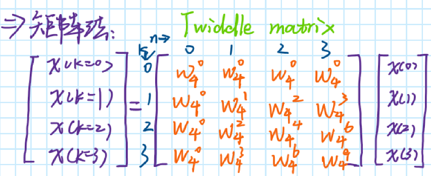
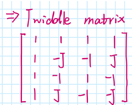
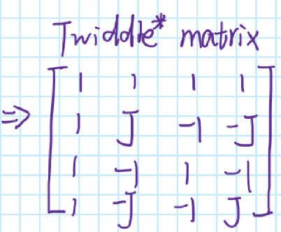
Rotation matrix of inverse DFT transform(IDFT)
?
Properties of DFT
1.linear
X 1 ( k ) = D F T [ x 1 ( n ) ] X_1(k)=DFT[x_1(n)] X1?(k)=DFT[x1?(n)]
X 2 ( k ) = D F T [ x 2 ( n ) ] X_2(k)=DFT[x_2(n)] X2?(k)=DFT[x2?(n)]
D F T [ a x 1 ( n ) + b x 2 ( n ) ] = a X 1 ( k ) + b X 2 ( k ) DFT[ax_1(n)+bx_2(n)]=aX_1(k)+bX_2(k) DFT[ax1?(n)+bx2?(n)]=aX1?(k)+bX2?(k)
2.circular convolution
DFT: x [ n ] ? h [ n ] ? X [ k ] ? H [ k ] x[n]\circledast h[n]\Leftrightarrow X[k]·H[k] x[n]?h[n]?X[k]?H[k]
DFT: x [ n ] ? h [ n ] ? X [ k ] ? H [ k ] x[n]· h[n]\Leftrightarrow X[k]\circledast H[k] x[n]?h[n]?X[k]?H[k]
3.periodicity
D F T [ x ( n ) ] = x ( k ) DFT[x(n)] = x(k) DFT[x(n)]=x(k)
x ( n + N ) = x ( n ) x(n+N) = x(n) x(n+N)=x(n);for all n
x ( k + N ) = x ( k ) x(k+N) = x(k) x(k+N)=x(k);for all k
4.cyclic frequency shift
D F T [ x ( n ) e j 2 π N l n ] = x ( ( k ? l ) ) N DFT[x(n)e^{j\frac{2\pi}{N}ln}]=x((k-l))_N DFT[x(n)ejN2π?ln]=x((k?l))N?
(( )) is cyclic frequency
?
DTF calculates linear convolution and circular convolution
linear convilution
[ y ( n ) = x ( n ) ? h ( n ) ] [y(n) = x(n)*h(n)] [y(n)=x(n)?h(n)]
then the length of x(n) is L,and h(n) is M
the length of linear convolution: N = L + M -1
- filling the length of x(n) and h(n) to N (add 0)
- calculates DTF[x(n)] and DTF[h(n)]
- then$ y(k) = x(k)·h(k)$
- calculate I D F T [ Y ( k ) ] = y ( n ) IDFT[Y(k)] = y(n) IDFT[Y(k)]=y(n)
?
cyclical convolution
[ y ( n ) = x ( n ) ? h ( n ) ] [y(n) = x(n)\circledast h(n)] [y(n)=x(n)?h(n)]
then the length of x(n) is L,and h(n) is M(add 0)
the length of cyclical convolution is :N = max(L,M)
- filling the length of x(n) and h(n) to N
- calculates DTF[x(n)] and DTF[h(n)]
- then y ( k ) = x ( k ) ? h ( k ) y(k) = x(k)·h(k) y(k)=x(k)?h(k)
- calculate I D F T [ Y ( k ) ] = y ( n ) IDFT[Y(k)] = y(n) IDFT[Y(k)]=y(n)
?
another way to calculate linear convolution
- Overlap-Add and Overlap-Save
Overlap-Add
then the length of x k ( n ) x_k(n) xk?(n) ( x k ( n ) x_k(n) xk?(n) is not x ( n ) x(n) x(n)) is L,and h(n) is M
the length of convolution is :N = L + M - 1 (the size of N is depend on you)
eg: x ( n ) = { 3 , ? 1 , 0 , 1 , 3 , 2 , 0 , 1 , 2 , 1 } x(n) = \{ 3,-1,0,1,3,2,0,1,2,1\} x(n)={3,?1,0,1,3,2,0,1,2,1} h ( n ) = { 1 , 1 , 1 } h(n) = \{ 1,1,1\} h(n)={1,1,1}
1.we take N = 6,then 6= L + 3 - 1;so L = 4.
x 1 ( n ) = { 0 , 0 , 3 , ? 1 , 0 , 1 } x_1(n) = \{ 0,0,3,-1,0,1 \} x1?(n)={0,0,3,?1,0,1}
x 2 ( n ) = { 0 , 1 , 3 , 2 , 0 , 1 } x_2(n) = \{ 0,1,3,2 ,0,1\} x2?(n)={0,1,3,2,0,1}
x 3 ( n ) = { 0 , 1 , 2 , 1 , 0 , 0 } x_3(n) = \{ 0,1,2,1,0,0 \} x3?(n)={0,1,2,1,0,0}
h ( n ) = { 1 , 1 , 1 , 0 , 0 , 0 } h(n) = \{1,1,1,0,0,0\} h(n)={1,1,1,0,0,0}
2.calculate
x 1 ( n ) ? h ( n ) = { 1 , 1 , 3 , 2 , 2 , 0 } x_1(n)\circledast h(n) =\{1,1,3,2,2,0\} x1?(n)?h(n)={1,1,3,2,2,0}
x 2 ( n ) ? h ( n ) = { 1 , 2 , 4 , 6 , 5 , 3 } x_2(n)\circledast h(n)=\{1,2,4,6,5,3\} x2?(n)?h(n)={1,2,4,6,5,3}
x 3 ( n ) ? h ( n ) = { 0 , 1 , 3 , 4 , 3 , 1 } x_3(n)\circledast h(n) =\{0,1,3,4,3,1\} x3?(n)?h(n)={0,1,3,4,3,1}
3.Remove first (M-1) points ,Concatenate all results
the result is { 3 , 2 , 2 , 0 , 4 , 6 , 5 , 3 , 3 , 4 , 3 , 1 } \{3,2,2,0,4,6,5,3,3,4,3,1\} {3,2,2,0,4,6,5,3,3,4,3,1}
?
Overlap-Save
then the length of x k ( n ) x_k(n) xk?(n) ( x k ( n ) x_k(n) xk?(n) is not x ( n ) x(n) x(n)) is L,and h(n) is M
the length of convolution is :N = L + M - 1 (the size of N is depend on you)
eg: x ( n ) = { 3 , ? 1 , 0 , 1 , 3 , 2 , 0 , 1 , 2 , 1 } x(n) = \{ 3,-1,0,1,3,2,0,1,2,1\} x(n)={3,?1,0,1,3,2,0,1,2,1} h ( n ) = { 1 , 1 , 1 } h(n) = \{ 1,1,1\} h(n)={1,1,1}
1.we take N = 5,then 5 = L + 3 - 1;so L = 3.
x 1 ( n ) = { 0 , 0 , 3 , ? 1 , 0 } x_1(n) = \{ 0,0,3,-1,0 \} x1?(n)={0,0,3,?1,0}
x 2 ( n ) = { ? 1 , 0 , 1 , 3 , 2 } x_2(n) = \{ -1,0,1,3,2 \} x2?(n)={?1,0,1,3,2}
x 3 ( n ) = { 3 , 2 , 0 , 1 , 2 } x_3(n) = \{ 3,2,0,1,2 \} x3?(n)={3,2,0,1,2}
x 4 ( n ) = { 1 , 2 , 1 , 0 , 0 } x_4(n) = \{ 1,2,1,0,0 \} x4?(n)={1,2,1,0,0}
h ( n ) = { 1 , 1 , 1 , 0 , 0 } h(n) = \{1,1,1,0,0\} h(n)={1,1,1,0,0}
2.calculate
x 1 ( n ) ? h ( n ) = { ? 1 , 0 , 3 , 2 , 2 } x_1(n)\circledast h(n) =\{-1,0,3,2,2\} x1?(n)?h(n)={?1,0,3,2,2}
x 2 ( n ) ? h ( n ) = { 4 , 1 , 0 , 4 , 6 } x_2(n)\circledast h(n)=\{4,1,0,4,6\} x2?(n)?h(n)={4,1,0,4,6}
x 3 ( n ) ? h ( n ) = { 6 , 7 , 5 , 3 , 3 } x_3(n)\circledast h(n) =\{6,7,5,3,3\} x3?(n)?h(n)={6,7,5,3,3}
x 4 ( n ) ? h ( n ) = { 1 , 3 , 4 , 3 , 1 } x_4(n)\circledast h(n) =\{1,3,4,3,1\} x4?(n)?h(n)={1,3,4,3,1}
3.Remove first (M-1) points ,Concatenate all results
the result is { 3 , 2 , 2 , 0 , 4 , 6 , 5 , 3 , 3 , 4 , 3 , 1 } \{3,2,2,0,4,6,5,3,3,4,3,1\} {3,2,2,0,4,6,5,3,3,4,3,1}
?
?
z-transformation
- Basic concepts of z-transformation
- ROC
- Properties of z-transformation
- Inverse transformation of z-transform
- stable
Basic concepts of z-transformation
-
Bilateral Z Transform
-
Unilateral Z Transform
Bilateral Z Transform:
X ( Z ) = Z { x [ n ] } = ∑ n = ? ∞ + ∞ x [ n ] Z ? n , Z ∈ R x X(Z)=Z\left\{x[n]\right\}=\sum_{n=-\infty}^{+\infty}x\left[n\right]Z^{-n}\text{,}Z\in Rx X(Z)=Z{x[n]}=∑n=?∞+∞?x[n]Z?n,Z∈Rx
Unilateral Z Transform:
X ( Z ) = Z { x [ n ] } = ∑ n = 0 + ∞ x [ n ] Z ? n , Z ∈ R x X(Z)=Z\left\{x[n]\right\}=\sum_{n=0}^{+\infty}x\left[n\right]Z^{-n},Z\in Rx X(Z)=Z{x[n]}=∑n=0+∞?x[n]Z?n,Z∈Rx
?
region of convergence (ROC)
making z = r ? e j w z = r·e^{jw} z=r?ejw
x ( z ) = ∑ n = ? ∞ ∞ x ( n ) z ? n = ∑ n = ? ∞ ∞ x ( n ) r ? n e ? j w n x(z) = \sum_{n=-\infty}^{\infty}x(n)z^{-n} \\=\sum_{n=-\infty}^{\infty}x(n)r^{-n}e^{-jwn} x(z)=∑n=?∞∞?x(n)z?n=∑n=?∞∞?x(n)r?ne?jwn
if r = 1 r = 1 r=1,then x ( z ) = D T F T x(z) = DTFT x(z)=DTFT
eg: x ( n ) = { 1 , 2 , 3 , 4 , 0 , 1 } x(n) = \{1,2,3,4,0,1 \} x(n)={1,2,3,4,0,1}
x ( z ) = ∑ n = ? ∞ ∞ x ( n ) z ? n = ∑ n = 0 5 x ( n ) z ? n = x ( 0 ) z ? 0 + x ( 1 ) z ? 1 + x ( 2 ) z ? 2 + x ( 3 ) z ? 3 + x ( 4 ) z ? 4 + x ( 5 ) z ? 5 = 1 + 2 z ? 1 + 3 z ? 2 + 4 z ? 3 + z ? 5 x(z) = \sum_{n=-\infty}^{\infty}x(n)z^{-n}=\sum_{n=0}^{5}x(n)z^{-n}=x(0)z^{-0}+x(1)z^{-1}+x(2)z^{-2}+x(3)z^{-3}+x(4)z^{-4}+x(5)z^{-5}\\=1+2z^{-1}+3z^{-2}+4z^{-3}+z^{-5} x(z)=∑n=?∞∞?x(n)z?n=∑n=05?x(n)z?n=x(0)z?0+x(1)z?1+x(2)z?2+x(3)z?3+x(4)z?4+x(5)z?5=1+2z?1+3z?2+4z?3+z?5
ROC:exist entire z-plane except z = 0 z = 0 z=0
using plot:
eg: x ( n ) = { a n ?? ; n ? ≥ 0 0 ?? ; n ? < 0 x(n)=\left\{\begin{matrix} a^n\;;n\ \ge 0 \\ 0\;;n\ < 0 \end{matrix}\right. x(n)={an;n?≥00;n?<0?
x ( z ) = ∑ n = 0 + ∞ ( a z ? 1 ) n = 1 1 ? a z ? 1 = z z ? a x(z) = \sum_{n=0}^{+\infty}(az^{-1})^{n}\\=\frac{1}{1-az^{-1}}=\frac{z}{z-a} x(z)=∑n=0+∞?(az?1)n=1?az?11?=z?az?
needing that : ∣ a z ? 1 ∣ < 1 |az^{-1}|<1 ∣az?1∣<1 just ROC: ∣ z ∣ > ∣ a ∣ |z|> |a| ∣z∣>∣a∣
eg : x ( n ) = ? a n u ( ? n ? 1 ) x(n) = -a^nu(-n-1) x(n)=?anu(?n?1)
ROC: ∣ a ? 1 ∣ < 1 |a^{-1}|<1 ∣a?1∣<1 is just ∣ z ∣ < ∣ a ∣ |z| < |a| ∣z∣<∣a∣
?
Properties of z-transformation
- linear
- time shifting
- scaling
- differential
- convolution
- initial value theorem
- terminal value theorem
linear
x 1 ( n ) ? x 1 ( z ) ; R O C 1 x_1(n) \longrightarrow x_1(z);ROC_1 x1?(n)?x1?(z);ROC1?
x 2 ( n ) ? x 2 ( z ) ; R O C 2 x_2(n) \longrightarrow x_2(z);ROC_2 x2?(n)?x2?(z);ROC2?
a x 1 ( n ) + b x 2 ( n ) ? a x 1 ( z ) + b x 2 ( z ) ; R O C : [ R O C 1 ∩ R O C 2 ] ax_1(n) + bx_2(n) \longrightarrow ax_1(z)+bx_2(z);\\ROC:[ROC_1\cap ROC_2] ax1?(n)+bx2?(n)?ax1?(z)+bx2?(z);ROC:[ROC1?∩ROC2?]
time shifting
x ( n ) ? x ( z ) x(n) \longrightarrow x(z) x(n)?x(z)
x ( n ? n 0 ) ? x ( z ) z ? n 0 x(n - n_0) \longrightarrow x(z)z^{-n_0} x(n?n0?)?x(z)z?n0?
scaling
x ( n ) ? x ( z ) ; R O C : ?? ∣ z ∣ > 1 x(n) \longrightarrow x(z);ROC: \;|z|>1 x(n)?x(z);ROC:∣z∣>1
a n x ( n ) ? x ( z a ) a^nx(n) \longrightarrow x(\frac{z}{a}) anx(n)?x(az?)
differential
x ( n ) ? x ( z ) x(n) \longrightarrow x(z) x(n)?x(z)
n x ( n ) ? ? z d x ( z ) d z nx(n) \longrightarrow -z \frac{dx(z)}{dz} nx(n)??zdzdx(z)?
convolution
x 1 ( n ) ? x 2 ( n ) ? x 1 ( z ) ? x 2 ( z ) x_1(n) * x_2(n) \longrightarrow x_1(z)·x_2(z) x1?(n)?x2?(n)?x1?(z)?x2?(z)
initial value theorem
x ( 0 ) = lim ? n → 0 x ( n ) = lim ? z → + ∞ x ( z ) x(0) = \lim_{n \to 0}x(n) = \lim_{z \to +\infty}x(z) x(0)=limn→0?x(n)=limz→+∞?x(z)
terminal value theorem
x ( + ∞ ) = lim ? n → ∞ x ( n ) = lim ? z → 1 ( 1 ? z ? 1 ) x ( z ) x(+\infty) = \lim_{n \to \infty}x(n) = \lim_{z \to 1}(1-z^{-1})x(z) x(+∞)=limn→∞?x(n)=limz→1?(1?z?1)x(z)
?
Inverse transformation of z-transform
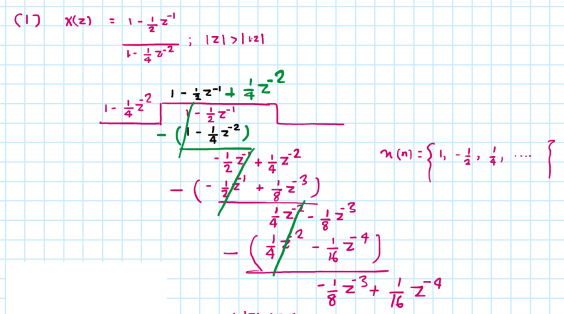
- long division method
- partial fraction expansion method
- Residue method
long division method
partial fraction expansion method
x ( z ) = z ( z ? 1 2 ) ( z + 1 2 ) ( z + 1 4 ) x(z) = \frac{z(z-\frac{1}{2})}{(z+\frac{1}{2})(z+\frac{1}{4})} x(z)=(z+21?)(z+41?)z(z?21?)?
x ( z ) z = z ? 1 2 ( z + 1 2 ) ( z + 1 4 ) = 4 z + 1 2 ? 3 z + 1 4 \frac{x(z)}{z} = \frac{z-\frac{1}{2}}{(z+\frac{1}{2})(z+\frac{1}{4})}=\frac{4}{z+\frac{1}{2}}-\frac{3}{z+\frac{1}{4}} zx(z)?=(z+21?)(z+41?)z?21??=z+21?4??z+41?3?
x ( z ) = 4 z z + 1 2 ? 3 z z + 1 4 x(z) = \frac{4z}{z+\frac{1}{2}} - \frac{3z}{z+\frac{1}{4}} x(z)=z+21?4z??z+41?3z?
x ( n ) = 4 ( ? 1 2 ) n u ( n ) ? 3 ( ? 1 4 ) n u ( n ) x(n) = 4(-\frac{1}{2})^{n}u(n) -3 (-\frac{1}{4})^{n}u(n) x(n)=4(?21?)nu(n)?3(?41?)nu(n)
Residue method
x ( z ) = 1 ( z ? 2 ) ( z ? 3 ) x(z) = \frac{1}{(z-2)(z-3)} x(z)=(z?2)(z?3)1?
1. z n ? 1 x ( z ) = z n ? 1 ( z ? 2 ) ( z ? 3 ) z^{n-1}x(z) = \frac{z^{n-1}}{(z-2)(z-3)} zn?1x(z)=(z?2)(z?3)zn?1?
2. R 1 = ( z ? 2 ) z n ? 1 ( z ? 2 ) ( z ? 3 ) ∣ z = 2 = ? 2 n ? 1 R_1 =(z-2)\frac{z^{n-1}}{(z-2)(z-3)}|_{z=2} = -2^{n-1} R1?=(z?2)(z?2)(z?3)zn?1?∣z=2?=?2n?1
3. R 2 = ( z ? 3 ) z n ? 1 ( z ? 2 ) ( z ? 3 ) ∣ z = 3 = 3 n ? 1 R_2 =(z-3)\frac{z^{n-1}}{(z-2)(z-3)}|_{z=3} = 3^{n-1} R2?=(z?3)(z?2)(z?3)zn?1?∣z=3?=3n?1
4. x ( n ) = ? 2 n ? 1 + 3 n ? 1 x(n) = -2^{n-1} + 3^{n-1} x(n)=?2n?1+3n?1
?
stability
S = ∑ k = ? ∞ ∞ ∣ h ( n ) ∣ < + ∞ S=\sum_{k=-\infty}^{\infty}|h(n)| < +\infty S=∑k=?∞∞?∣h(n)∣<+∞
本文来自互联网用户投稿,该文观点仅代表作者本人,不代表本站立场。本站仅提供信息存储空间服务,不拥有所有权,不承担相关法律责任。 如若内容造成侵权/违法违规/事实不符,请联系我的编程经验分享网邮箱:veading@qq.com进行投诉反馈,一经查实,立即删除!