非均衡设计评价两个批次的数据一致性

任务描述

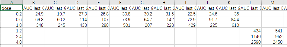
第一批次的药物实验设置了三个剂量（0.2，0.6，1.8）mg/kg，每个剂量水平有十个受试者。
第二批次的药物实验设置了其他三个剂量(1.2,2.4,4.8) mk/kg，每个剂量水平有两个受试者。
问：这两个数据一致性怎么样？

其实我不理解这个一致性如何评价！！！
我理解是不是这两批数据可以用一个方程表示？或者说第二批次数据落在第一批次方程的置信区间内？

数据

getwd()
rm(list=ls())
list.files()
library(tidyverse)

df <- read.table("AUClast1.csv",header = T,sep=",",encoding = "UTF-8")
head(df)

代码

# 重新整理一下数据
dose <- as.numeric(df[,1])
resp <- c(27.33,88.06,351.4,487.5,1046,2520)
df <- as.data.frame(cbind(dose,resp))
df <- df %>% arrange(dose)
head(df)
#  dose    resp
#1  0.2   27.33
#2  0.6   88.06
#3  1.2  487.50
#4  1.8  351.40
#5  2.4 1046.00
#6  4.8 2520.00

plot(log10(dose),log10(resp))

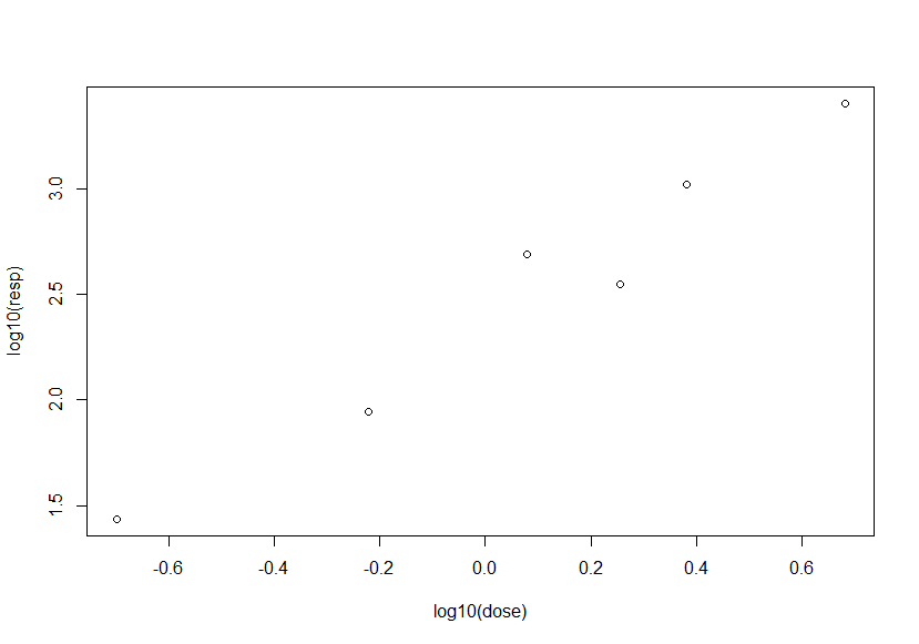
# 散点图可以看到数据取log后基本上是线性相关的，那就做线性拟合好了
# 然后第一批次的数据就三个点，什么正态分布，方差齐性，强影响点，都不考虑了，直接干
# 把第一批的数据拿出来
df1 <- df[c(1,2,4),]

model <- lm(log10(resp)~log10(dose),df1)
summary(model)
# 模型的截距和系数都有意义，继续

Call:
lm(formula = log10(resp) ~ log10(dose), data = df1
Residuals:
1 2 4
0.0155 -0.0310 0.0155
Coefficients:
Estimate Std. Error t value Pr(>|t|)
(Intercept) 2.2336 0.0252 88.7 0.0072
log10(dose) 1.1623 0.0562 20.7 0.0308
Residual standard error: 0.0379 on 1 degrees of freedom
Multiple R-squared: 0.998, Adjusted R-squared: 0.995
F-statistic: 428 on 1 and 1 DF, p-value: 0.0308

# 用上面的模型预测六个剂量水平的响应值，以及95%的置信区间
p1 <- predict(model,df,interval = "confidence", level = 0.95)
p1
#  fit    lwr   upr
#1 1.421 0.9813 1.861
#2 1.976 1.6976 2.254
#3 2.326 1.9741 2.677
#4 2.530 2.0905 2.970
#5 2.676 2.1635 3.188
#6 3.025 2.3231 3.728

# 把dose，response，fit，lwr，upr构造一个数据框作图
df <- cbind(df,p1)
df %>% 
  ggplot(aes(x = log10(dose), y = log10(resp))) +
  geom_point(colour = "midnightblue", alpha = 0.5,size=1) +
  geom_line(aes(y = lwr), lty = 2,color = "blue") +
  geom_line(aes(y = upr), lty = 2,color = "green") +
  labs(x = "log10(Dose)", y = "log10(Response)", color = NULL) +
  theme_test() 

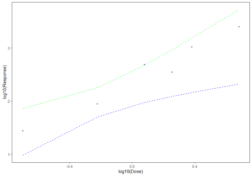
# 置信区间用色带表示
# 坐标轴改一下
# fit值用红线表示
# 真实数据点 用散点表示
dose02 <- as.numeric(df[1,2:11])
dose06 <- as.numeric(df[2,2:11])
dose18 <- as.numeric(df[3,2:11])
dose12 <- as.numeric(df[4,12:13])
dose24 <- as.numeric(df[5,12:13])
dose48 <- as.numeric(df[6,12:13])
df2 <- cbind(rep(0.2,10),dose02)
df2 <- rbind(df2,cbind(rep(0.6,10),dose06))
df2 <- rbind(df2,cbind(rep(1.2,2),dose12))
df2 <- rbind(df2,cbind(rep(1.8,10),dose18))
df2 <- rbind(df2,cbind(rep(2.4,2),dose24))
df2 <- rbind(df2,cbind(rep(4.8,2),dose48))
df2 <- as.data.frame(df2)
colnames(df2) <- c("dose","resp")
df <- merge(df2,df,all.x = T,by = "dose")

xlabs <- unique(df$dose)
ylabs <- unique(df$resp.y)
head(df,10)
#  dose resp.x resp.y   fit    lwr   upr
#1   0.2   24.9  27.33 1.421 0.9813 1.861
#2   0.2   19.7  27.33 1.421 0.9813 1.861
#3   0.2   27.3  27.33 1.421 0.9813 1.861
#4   0.2   26.8  27.33 1.421 0.9813 1.861
#5   0.2   30.8  27.33 1.421 0.9813 1.861
#6   0.2   30.2  27.33 1.421 0.9813 1.861
#7   0.2   31.5  27.33 1.421 0.9813 1.861
#8   0.2   22.5  27.33 1.421 0.9813 1.861
#9   0.2   24.6  27.33 1.421 0.9813 1.861
#10  0.2   35.0  27.33 1.421 0.9813 1.861

df %>% 
  ggplot(aes(x = log10(dose), y = fit)) +
  geom_line(colour = "red", alpha = 0.5) +
  geom_point(aes( y = log10(resp.x)),color="darkblue")+
  geom_ribbon(aes(ymin = lwr, ymax = upr), fill = "blue", alpha = 0.3)+
  labs(x = "Dose,mg/kg", y = "AUG_last.(h*ug/mL)", color = NULL) +
  scale_x_continuous(breaks = log10(xlabs),labels = xlabs)+
  scale_y_continuous(breaks = log10(ylabs),labels = ylabs)+
  theme_test()+
  labs(title = "AUC-dose relationship")

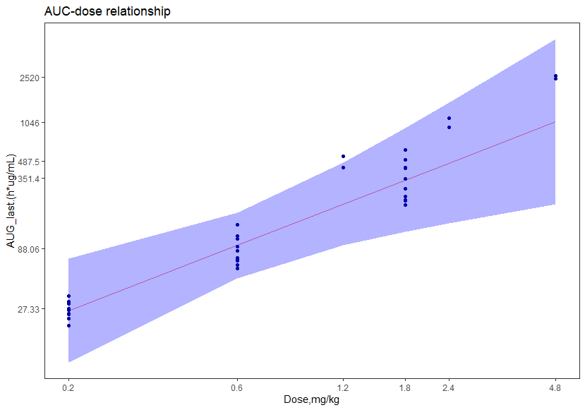
结论

使用第一批数据拟合的方程，用于预测第二批次数据，使用第二批次的剂量作为因变量，在95%的置信区间内，第二批次的response落在了预测区间内。
凑合能说第二个批次的数据 与 第一批数据具有一致性。