从零开始的神经网络

先决条件

在本文中，我将解释如何通过实现前向和后向传递（反向传播）来构建基本的深度神经网络。这需要一些关于神经网络功能的具体知识。

了解线性代数的基础知识也很重要，这样才能理解我为什么要在本文中执行某些运算。我最好的建议是看 3Blue1Brown 的系列线性代数的本质.

NumPy

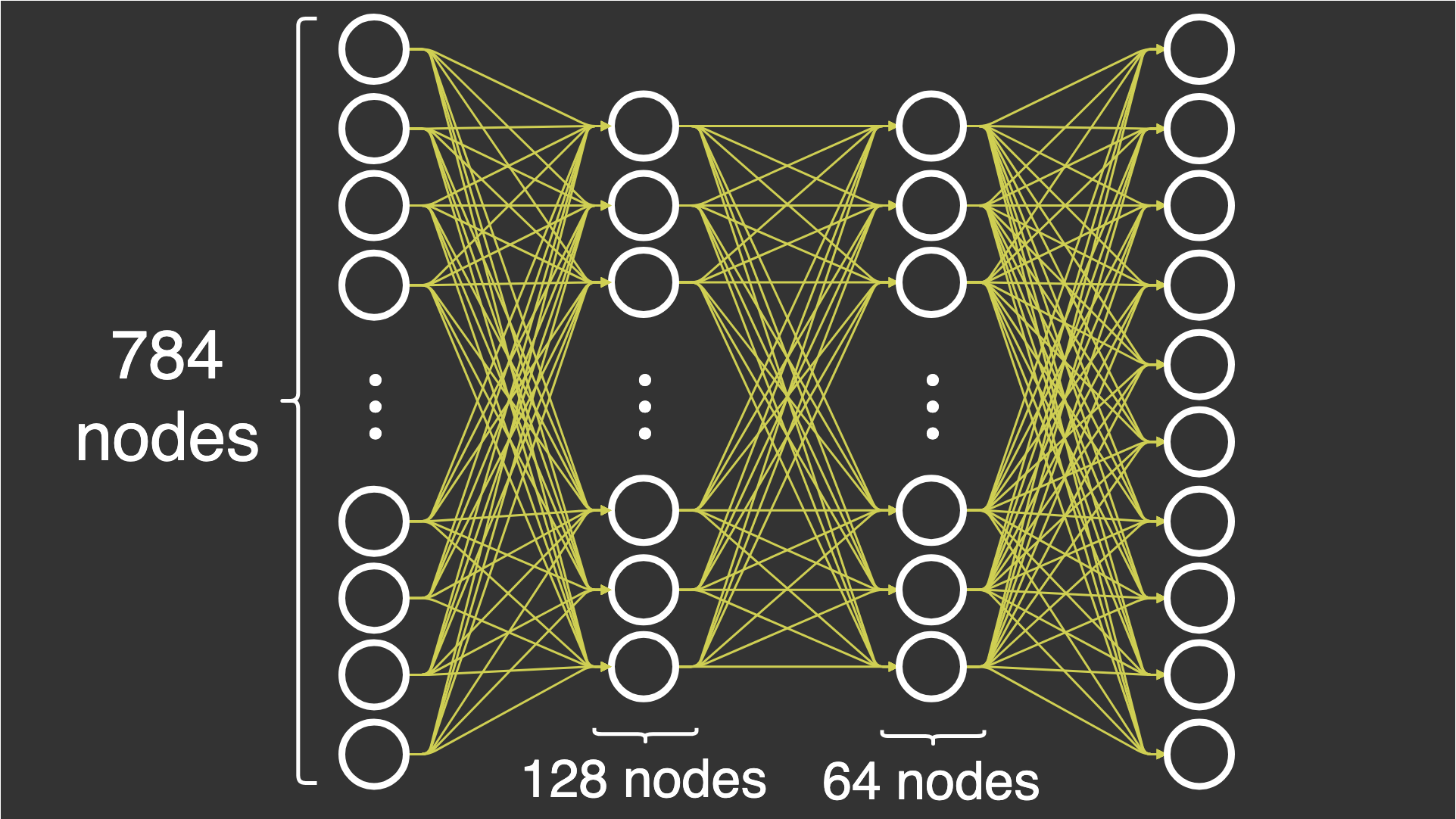
在本文中，我构建了一个包含 4 层的基本深度神经网络：1 个输入层、2 个隐藏层和 1 个输出层。所有层都是完全连接的。我正在尝试使用一个名为MNIST.该数据集由 70,000 张图像组成，每张图像的尺寸为 28 x 28 像素。数据集包含每个图像的一个标签，该标签指定我在每张图像中看到的数字。我说有 10 个类，因为我有 10 个标签。

MNIST 数据集中的 10 个数字示例，放大 2 倍

为了训练神经网络，我使用随机梯度下降，这意味着我一次将一张图像通过神经网络。

让我们尝试以精确的方式定义图层。为了能够对数字进行分类，在运行神经网络后，您必须最终获得属于某个类别的图像的概率，因为这样您就可以量化神经网络的性能。

1. 输入层：在此层中，我输入由 28x28 图像组成的数据集。我将这些图像展平成一个包含 28×28=78428×28=784 个元素的数组。这意味着输入层将有 784 个节点。

2. 隐藏层 1：在此层中，我将输入层中的节点数从 784 个减少到 128 个节点。当你在神经网络中前进时，这会带来一个挑战（我稍后会解释这一点）。

3. 隐藏层 2：在这一层中，我决定从第一个隐藏层的 128 个节点开始使用 64 个节点。这并不是什么新挑战，因为我已经减少了第一层的数量。

4. 输出层：在这一层中，我将 64 个节点减少到总共 10 个节点，以便我可以根据标签评估节点。此标签以包含 10 个元素的数组的形式接收，其中一个元素为 1，其余元素为 0。

您可能意识到，每层中的节点数从 784 个节点减少到 128 个节点，从 64 个节点减少到 10 个节点。这是基于经验观察这会产生更好的结果，因为我们既没有过度拟合，也没有过度拟合，只是试图获得正确数量的节点。本文选择的具体节点数是随机选择的，但为了避免过度拟合，节点数量会减少。在大多数现实生活中，您可能希望通过蛮力或良好的猜测（通常是通过网格搜索或随机搜索）来优化这些参数，但这超出了本文的讨论范围。

导入和数据集

对于整个 NumPy 部分，我特别想分享使用的导入。请注意，我使用 NumPy 以外的库来更轻松地加载数据集，但它们不用于任何实际的神经网络。

from sklearn.datasets import fetch_openml
from keras.utils.np_utils import to_categorical
import numpy as np
from sklearn.model_selection import train_test_split
import time

现在，我必须加载数据集并对其进行预处理，以便可以在 NumPy 中使用它。我通过将所有图像除以 255 来进行归一化，并使所有图像的值都在 0 - 1 之间，因为这消除了以后激活函数的一些数值稳定性问题。我使用独热编码标签，因为我可以更轻松地从神经网络的输出中减去这些标签。我还选择将输入加载为 28 * 28 = 784 个元素的扁平化数组，因为这是输入层所需要的。

x, y = fetch_openml('mnist_784', version=1, return_X_y=True)
x = (x/255).astype('float32')
y = to_categorical(y)
?
x_train, x_val, y_train, y_val = train_test_split(x, y, test_size=0.15, random_state=42)

初始化

神经网络中权重的初始化有点难考虑。要真正理解以下方法的工作原理和原因，您需要掌握线性代数，特别是使用点积运算时的维数。

尝试实现前馈神经网络时出现的具体问题是，我们试图从 784 个节点转换为 10 个节点。在实例化类时，我传入一个大小数组，该数组定义了每一层的激活次数。DeepNeuralNetwork

dnn = DeepNeuralNetwork(sizes=[784, 128, 64, 10])

这将通过函数初始化类。

DeepNeuralNetwork``init

def __init__(self, sizes, epochs=10, l_rate=0.001):
 ?  self.sizes = sizes
 ?  self.epochs = epochs
 ?  self.l_rate = l_rate
?
 ?  # we save all parameters in the neural network in this dictionary
 ?  self.params = self.initialization()

让我们看看在调用函数时大小如何影响神经网络的参数。我正在准备“可点”的 m x n 矩阵，以便我可以进行前向传递，同时随着层的增加减少激活次数。我只能对两个矩阵 M1 和 M2 使用点积运算，其中 M1 中的 m 等于 M2 中的 n，或者 M1 中的 n 等于 M2 中的 m。initialization()

通过这个解释，您可以看到我用 m=128m=128 和 n=784n=784 初始化了第一组权重 W1，而接下来的权重 W2 是 m=64m=64 和 n=128n=128。如前所述，输入层 A0 中的激活次数等于 784，当我将激活 A0 点在 W1 上时，操作成功。

def initialization(self):
 ?  # number of nodes in each layer
 ?  input_layer=self.sizes[0]
 ?  hidden_1=self.sizes[1]
 ?  hidden_2=self.sizes[2]
 ?  output_layer=self.sizes[3]
?
 ?  params = {
 ? ? ?  'W1':np.random.randn(hidden_1, input_layer) * np.sqrt(1. / hidden_1),
 ? ? ?  'W2':np.random.randn(hidden_2, hidden_1) * np.sqrt(1. / hidden_2),
 ? ? ?  'W3':np.random.randn(output_layer, hidden_2) * np.sqrt(1. / output_layer)
 ?  }
?
 ?  return params

前馈

前向传递由 NumPy 中的点运算组成，结果证明它只是矩阵乘法。我必须将权重乘以前一层的激活。然后，我必须将激活函数应用于结果。

为了完成每一层，我依次应用点运算，然后应用 sigmoid 激活函数。在最后一层中，我使用激活函数，因为我想拥有每个类的概率，以便我可以测量当前前向传递的性能。softmax

注意：我选择了该函数的数值稳定版本。您可以从斯坦福大学的课程中阅读更多内容softmaxCS231n.

def initialization(self):
 ?  # number of nodes in each layer
 ?  input_layer=self.sizes[0]
 ?  hidden_1=self.sizes[1]
 ?  hidden_2=self.sizes[2]
 ?  output_layer=self.sizes[3]
?
 ?  params = {
 ? ? ?  'W1':np.random.randn(hidden_1, input_layer) * np.sqrt(1. / hidden_1),
 ? ? ?  'W2':np.random.randn(hidden_2, hidden_1) * np.sqrt(1. / hidden_2),
 ? ? ?  'W3':np.random.randn(output_layer, hidden_2) * np.sqrt(1. / output_layer)
 ?  }
?
 ?  return params

以下代码显示了本文中使用的激活函数。可以看出，我提供了 sigmoid 的衍生版本，因为稍后通过神经网络反向传播时需要它。

def sigmoid(self, x, derivative=False):
 ?  if derivative:
 ? ? ?  return (np.exp(-x))/((np.exp(-x)+1)**2)
 ?  return 1/(1 + np.exp(-x))
?
def softmax(self, x):
 ?  # Numerically stable with large exponentials
 ?  exps = np.exp(x - x.max())
 ?  return exps / np.sum(exps, axis=0)

反向传播

向后传递很难正确，因为必须对齐的大小和操作才能使所有操作成功。这是向后传递的完整功能。我在下面介绍每个重量更新。

def backward_pass(self, y_train, output):
 ?  '''
 ? ? ?  This is the backpropagation algorithm, for calculating the updates
 ? ? ?  of the neural network's parameters.
 ?  '''
 ?  params = self.params
 ?  change_w = {}
?
 ?  # Calculate W3 update
 ?  error = output - y_train
 ?  change_w['W3'] = np.dot(error, params['A3'])
?
 ?  # Calculate W2 update
 ?  error = np.multiply( np.dot(params['W3'].T, error), self.sigmoid(params['Z2'], derivative=True) )
 ?  change_w['W2'] = np.dot(error, params['A2'])
?
 ?  # Calculate W1 update
 ?  error = np.multiply( np.dot(params['W2'].T, error), self.sigmoid(params['Z1'], derivative=True) )
 ?  change_w['W1'] = np.dot(error, params['A1'])
?
 ?  return change_w

W3 更新

的更新可以通过减去具有从称为 的前向传递的输出中调用的标签的真值数组来计算。此操作成功，因为是 10 并且也是 10。下面的代码可能是一个示例，其中 1 对应于 .W3``y_train``output``len(y_train)``len(output)``y_train``output

y_train = np.array([0, 0, 1, 0, 0, 0, 0, 0, 0, 0])

下面的代码显示了一个示例，其中数字是对应于 的类的概率。output``y_train

output = np.array([0.2, 0.2, 0.5, 0.3, 0.6, 0.4, 0.2, 0.1, 0.3, 0.7])

如果减去它们，则得到以下结果。

>>> output - y_train
array([ 0.2,  0.2, -0.5,  0.3,  0.6,  0.4,  0.2,  0.1,  0.3,  0.7])

下一个操作是点操作，它将错误（我刚刚计算的）与最后一层的激活点在一起。

error = output - y_train
change_w['W3'] = np.dot(error, params['A3'])

W2 更新

接下来是更新权重。为了成功，需要涉及更多的操作。首先，形状略有不匹配，因为具有形状和具有，即完全相同的尺寸。因此，我可以使用W2``W3``(10, 64)``error``(10, 64)转置操作这样数组的维度就会置换，并且形状现在会对齐以进行点操作。W3``.T

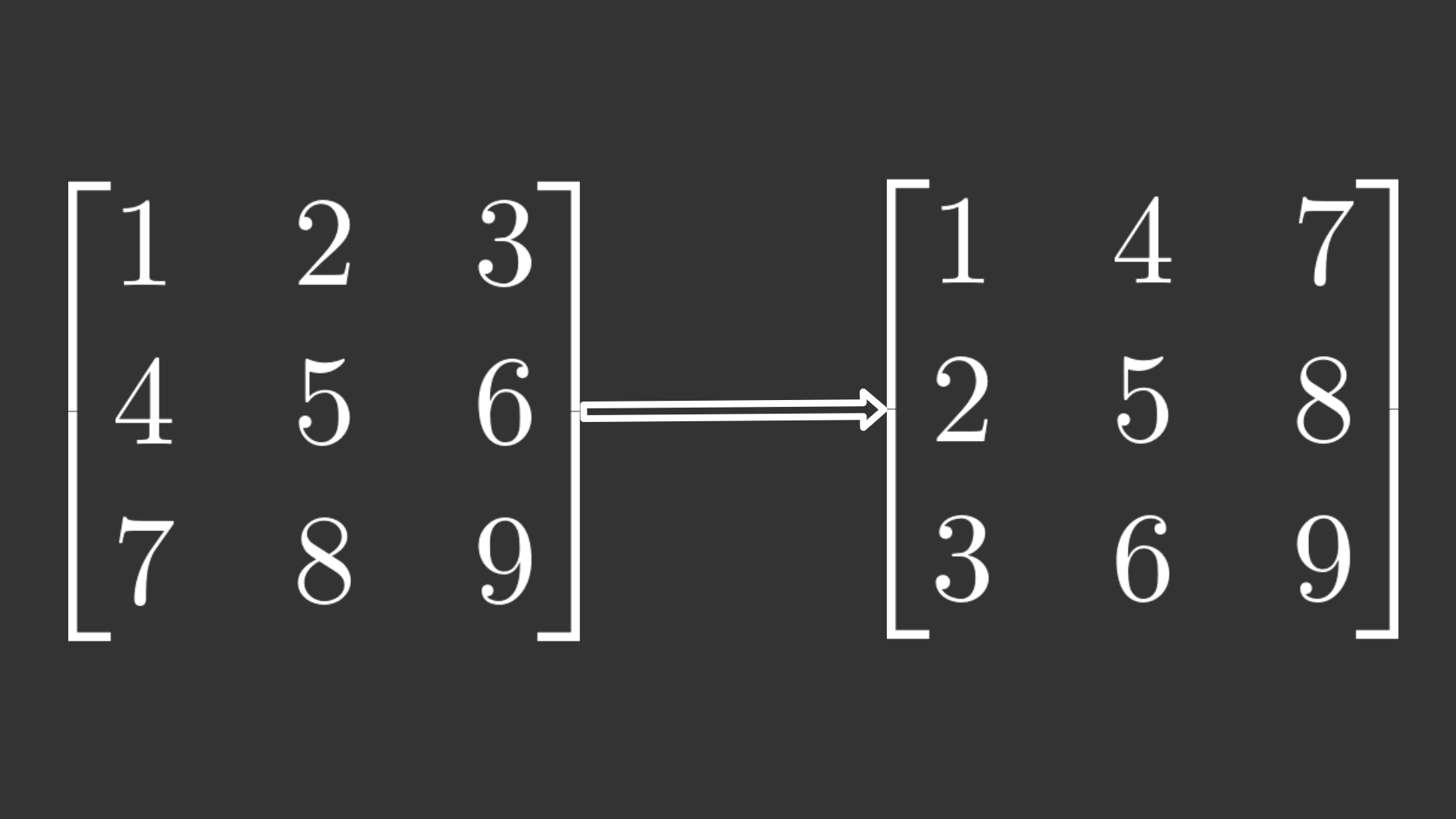
转置操作的示例。左：原始矩阵。右：置换矩阵

W3`现在有 shape 和 has shape ，它们与点运算兼容。结果是`(64, 10)``error``(10, 64)`[逐个元素相乘](https://docs.scipy.org/doc/numpy/reference/generated/numpy.multiply.html)（也称为 Hadamard 积）与 的 sigmoid 函数的导数的结果。最后，我将错误与上一层的激活点在一起。`Z2
error = np.multiply( np.dot(params['W3'].T, error), self.sigmoid(params['Z2'], derivative=True) )
change_w['W2'] = np.dot(error, params['A2'])

W1 更新

同样，用于更新的代码提前一步使用神经网络的参数。除其他参数外，代码等同于 W2 更新。W1

error = np.multiply( np.dot(params['W2'].T, error), self.sigmoid(params['Z1'], derivative=True) )
change_w['W1'] = np.dot(error, params['A1'])

训练（随机梯度下降）

我已经定义了向前和向后传递，但如何开始使用它们？我必须创建一个训练循环，并使用随机梯度下降 （SGD） 作为优化器来更新神经网络的参数。训练函数中有两个主要循环。一个循环表示 epoch 数，即我遍历整个数据集的次数，第二个循环用于逐个遍历每个观察值。

对于每个观测值，我都会使用 进行前向传递，这是数组中长度为 784 的一张图像，如前所述。前向传递的 与 一起使用，后者是后向传递中的独热编码标签（真实值）。这给了我一本关于神经网络中权重更新的字典。x``output``y

def train(self, x_train, y_train, x_val, y_val):
 ?  start_time = time.time()
 ?  for iteration in range(self.epochs):
 ? ? ?  for x,y in zip(x_train, y_train):
 ? ? ? ? ?  output = self.forward_pass(x)
 ? ? ? ? ?  changes_to_w = self.backward_pass(y, output)
 ? ? ? ? ?  self.update_network_parameters(changes_to_w)
?
 ? ? ?  accuracy = self.compute_accuracy(x_val, y_val)
 ? ? ?  print('Epoch: {0}, Time Spent: {1:.2f}s, Accuracy: {2}'.format(
 ? ? ? ? ?  iteration+1, time.time() - start_time, accuracy
 ? ? ?  ))

该函数具有 SGD 更新规则的代码，该规则只需要权重的梯度作为输入。需要明确的是，SGD 涉及使用来自后向传递的反向传播来计算梯度，而不仅仅是更新参数。它们似乎是分开的，应该分开考虑，因为这两种算法是不同的。update_network_parameters()

def update_network_parameters(self, changes_to_w):
 ?  '''
 ? ? ?  Update network parameters according to update rule from
 ? ? ?  Stochastic Gradient Descent.
?
 ? ? ?  θ = θ - η * ?J(x, y),
 ? ? ? ? ?  theta θ: ? ? ? ? ?  a network parameter (e.g. a weight w)
 ? ? ? ? ?  eta η: ? ? ? ? ? ?  the learning rate
 ? ? ? ? ?  gradient ?J(x, y):  the gradient of the objective function,
 ? ? ? ? ? ? ? ? ? ? ? ? ? ? ?  i.e. the change for a specific theta θ
 ?  '''
?
 ?  for key, value in changes_to_w.items():
 ? ? ?  for w_arr in self.params[key]:
 ? ? ? ? ?  w_arr -= self.l_rate * value

在更新了神经网络的参数后，我可以测量我之前准备的验证集的准确性，以验证网络在整个数据集上的每次迭代后的性能。

以下代码使用一些与训练函数相同的部分。首先，它进行前向传递，然后找到网络的预测，并检查与标签是否相等。之后，我将预测结果相加并除以 100 以找到准确性。接下来，我平均每个类的准确性。

def compute_accuracy(self, x_val, y_val):
 ?  '''
 ? ? ?  This function does a forward pass of x, then checks if the indices
 ? ? ?  of the maximum value in the output equals the indices in the label
 ? ? ?  y. Then it sums over each prediction and calculates the accuracy.
 ?  '''
 ?  predictions = []
?
 ?  for x, y in zip(x_val, y_val):
 ? ? ?  output = self.forward_pass(x)
 ? ? ?  pred = np.argmax(output)
 ? ? ?  predictions.append(pred == y)
?
 ?  summed = sum(pred for pred in predictions) / 100.0
 ?  return np.average(summed)

最后，在知道会发生什么之后，我可以调用训练函数。我使用训练和验证数据作为训练函数的输入，然后等待。

dnn.train(x_train, y_train, x_val, y_val)

请注意，结果可能会有很大差异，具体取决于权重的初始化方式。我的结果准确率为0%-95%。

以下是概述所发生情况的完整代码。

from sklearn.datasets import fetch_openml
from keras.utils.np_utils import to_categorical
import numpy as np
from sklearn.model_selection import train_test_split
import time
?
x, y = fetch_openml('mnist_784', version=1, return_X_y=True)
x = (x/255).astype('float32')
y = to_categorical(y)
?
x_train, x_val, y_train, y_val = train_test_split(x, y, test_size=0.15, random_state=42)
?
class DeepNeuralNetwork():
 ?  def __init__(self, sizes, epochs=10, l_rate=0.001):
 ? ? ?  self.sizes = sizes
 ? ? ?  self.epochs = epochs
 ? ? ?  self.l_rate = l_rate
?
 ? ? ?  # we save all parameters in the neural network in this dictionary
 ? ? ?  self.params = self.initialization()
?
 ?  def sigmoid(self, x, derivative=False):
 ? ? ?  if derivative:
 ? ? ? ? ?  return (np.exp(-x))/((np.exp(-x)+1)**2)
 ? ? ?  return 1/(1 + np.exp(-x))
?
 ?  def softmax(self, x):
 ? ? ?  # Numerically stable with large exponentials
 ? ? ?  exps = np.exp(x - x.max())
 ? ? ?  return exps / np.sum(exps, axis=0)
?
 ?  def initialization(self):
 ? ? ?  # number of nodes in each layer
 ? ? ?  input_layer=self.sizes[0]
 ? ? ?  hidden_1=self.sizes[1]
 ? ? ?  hidden_2=self.sizes[2]
 ? ? ?  output_layer=self.sizes[3]
?
 ? ? ?  params = {
 ? ? ? ? ?  'W1':np.random.randn(hidden_1, input_layer) * np.sqrt(1. / hidden_1),
 ? ? ? ? ?  'W2':np.random.randn(hidden_2, hidden_1) * np.sqrt(1. / hidden_2),
 ? ? ? ? ?  'W3':np.random.randn(output_layer, hidden_2) * np.sqrt(1. / output_layer)
 ? ? ?  }
?
 ? ? ?  return params
?
 ?  def forward_pass(self, x_train):
 ? ? ?  params = self.params
?
 ? ? ?  # input layer activations becomes sample
 ? ? ?  params['A0'] = x_train
?
 ? ? ?  # input layer to hidden layer 1
 ? ? ?  params['Z1'] = np.dot(params["W1"], params['A0'])
 ? ? ?  params['A1'] = self.sigmoid(params['Z1'])
?
 ? ? ?  # hidden layer 1 to hidden layer 2
 ? ? ?  params['Z2'] = np.dot(params["W2"], params['A1'])
 ? ? ?  params['A2'] = self.sigmoid(params['Z2'])
?
 ? ? ?  # hidden layer 2 to output layer
 ? ? ?  params['Z3'] = np.dot(params["W3"], params['A2'])
 ? ? ?  params['A3'] = self.softmax(params['Z3'])
?
 ? ? ?  return params['A3']
?
 ?  def backward_pass(self, y_train, output):
 ? ? ?  '''
 ? ? ? ? ?  This is the backpropagation algorithm, for calculating the updates
 ? ? ? ? ?  of the neural network's parameters.
?
 ? ? ? ? ?  Note: There is a stability issue that causes warnings. This is
 ? ? ? ? ? ? ? ?  caused  by the dot and multiply operations on the huge arrays.
?
 ? ? ? ? ? ? ? ?  RuntimeWarning: invalid value encountered in true_divide
 ? ? ? ? ? ? ? ?  RuntimeWarning: overflow encountered in exp
 ? ? ? ? ? ? ? ?  RuntimeWarning: overflow encountered in square
 ? ? ?  '''
 ? ? ?  params = self.params
 ? ? ?  change_w = {}
?
 ? ? ?  # Calculate W3 update
 ? ? ?  error = output - y_train
 ? ? ?  change_w['W3'] = np.dot(error, params['A3'])
?
 ? ? ?  # Calculate W2 update
 ? ? ?  error = np.multiply( np.dot(params['W3'].T, error), self.sigmoid(params['Z2'], derivative=True) )
 ? ? ?  change_w['W2'] = np.dot(error, params['A2'])
?
 ? ? ?  # Calculate W1 update
 ? ? ?  error = np.multiply( np.dot(params['W2'].T, error), self.sigmoid(params['Z1'], derivative=True) )
 ? ? ?  change_w['W1'] = np.dot(error, params['A1'])
?
 ? ? ?  return change_w
?
 ?  def update_network_parameters(self, changes_to_w):
 ? ? ?  '''
 ? ? ? ? ?  Update network parameters according to update rule from
 ? ? ? ? ?  Stochastic Gradient Descent.
?
 ? ? ? ? ?  θ = θ - η * ?J(x, y),
 ? ? ? ? ? ? ?  theta θ: ? ? ? ? ?  a network parameter (e.g. a weight w)
 ? ? ? ? ? ? ?  eta η: ? ? ? ? ? ?  the learning rate
 ? ? ? ? ? ? ?  gradient ?J(x, y):  the gradient of the objective function,
 ? ? ? ? ? ? ? ? ? ? ? ? ? ? ? ? ?  i.e. the change for a specific theta θ
 ? ? ?  '''
?
 ? ? ?  for key, value in changes_to_w.items():
 ? ? ? ? ?  for w_arr in self.params[key]:
 ? ? ? ? ? ? ?  w_arr -= self.l_rate * value
?
 ?  def compute_accuracy(self, x_val, y_val):
 ? ? ?  '''
 ? ? ? ? ?  This function does a forward pass of x, then checks if the indices
 ? ? ? ? ?  of the maximum value in the output equals the indices in the label
 ? ? ? ? ?  y. Then it sums over each prediction and calculates the accuracy.
 ? ? ?  '''
 ? ? ?  predictions = []
?
 ? ? ?  for x, y in zip(x_val, y_val):
 ? ? ? ? ?  output = self.forward_pass(x)
 ? ? ? ? ?  pred = np.argmax(output)
 ? ? ? ? ?  predictions.append(pred == y)
?
 ? ? ?  summed = sum(pred for pred in predictions) / 100.0
 ? ? ?  return np.average(summed)
?
 ?  def train(self, x_train, y_train, x_val, y_val):
 ? ? ?  start_time = time.time()
 ? ? ?  for iteration in range(self.epochs):
 ? ? ? ? ?  for x,y in zip(x_train, y_train):
 ? ? ? ? ? ? ?  output = self.forward_pass(x)
 ? ? ? ? ? ? ?  changes_to_w = self.backward_pass(y, output)
 ? ? ? ? ? ? ?  self.update_network_parameters(changes_to_w)
?
 ? ? ? ? ?  accuracy = self.compute_accuracy(x_val, y_val)
 ? ? ? ? ?  print('Epoch: {0}, Time Spent: {1:.2f}s, Accuracy: {2}'.format(
 ? ? ? ? ? ? ?  iteration+1, time.time() - start_time, accuracy
 ? ? ? ? ?  ))
?
dnn = DeepNeuralNetwork(sizes=[784, 128, 64, 10])
dnn.train(x_train, y_train, x_val, y_val)

NumPy 中的良好练习

您可能已经注意到，该代码的可读性很强，但它占用了大量空间，可以优化为循环运行。这是一个优化和改进它的机会。如果你是这个主题的新手，以下练习的难度很容易很难，最后一个练习是最难的。

1. 简单：实现 ReLU 激活函数或任何其他激活函数。检查 sigmoid 函数的实现方式以供参考，并记住实现导数。使用 ReLU 激活函数代替 sigmoid 函数。

2. 简单：初始化偏差并将它们添加到前向传递中的激活函数之前的 Z，并在后向传递中更新它们。当您尝试添加偏差时，请注意数组的维度。

3. 中：优化前向和后向传递，使它们在每个函数中循环运行。这使得代码更易于修改，并且可能更易于维护。for

   • 优化为神经网络进行权重的初始化函数，以便您可以在不使神经网络失败的情况下修改参数。sizes=[]

4. 中：实现小批量梯度下降，取代随机梯度下降。不要更新每个样品的参数，而是根据小批量中每个样品累积的梯度总和的平均值进行更新。小批量的大小通常在 64 以下。

5. 困难：实现 Adam 优化器。这应该在训练功能中实现。

   1. 通过添加额外的术语来实现 Momentum

   2. 基于 AdaGrad 优化器实现自适应学习率

   3. 结合步骤 1 和 2 来实现 Adam

我的信念是，如果你完成这些练习，你就会有一个良好的基础。下一步是实现卷积、滤波器等，但这留待以后的文章使用。

结论

本文介绍了如何在没有框架帮助的情况下构建神经网络的基础知识，这些框架可能使其更易于使用。我构建了一个具有 4 层的基本深度神经网络，并解释了如何通过实现前向和后向传递（反向传播）来构建基本的深度神经网络。