吴恩达深度学习l2week1编程作业—Gradient Checking（中文跑通版）

1.Packages

import numpy as np
from testCases import *
from public_tests import *
from gc_utils import sigmoid, relu, dictionary_to_vector, vector_to_dictionary, gradients_to_vector

%load_ext autoreload
%autoreload 2

2.问题描述

你是一个致力于在全球范围内提供移动支付的团队的一员，并被要求建立一个深度学习模型来检测欺诈行为——每当有人付款时，你都想看看付款是否可能是欺诈性的，比如用户的账户是否被黑客接管。

您已经知道，反向传播的实现非常具有挑战性，有时还会出现错误。因为这是一个任务关键型应用程序，您公司的首席执行官希望真正确定您的反向传播实施是正确的。你的首席执行官说：“给我证据，证明你的反向传播确实有效！”为了保证这一点，你将使用“梯度检查”

让我们来做吧！

3.Gradient Checking是如何工作的？

反向传播计算梯度𝐽?/𝐽𝜃,𝜃表示模型的参数。𝐽是使用前向传播和损失函数计算的。

𝐽是使用前向传播和损失函数计算的。因为前向传播相对容易实现，所以您确信自己做对了，因此您几乎100%确信自己正在计算成本𝐽正确地。因此，您可以使用代码进行计算𝐽验证用于计算的代码𝐽?/𝐽𝜃

标黄的地方是目的

4.一维梯度检查

Exercise 1 - forward_propagation

实现正向传播。对于这个简单的函数计算𝐽（.）

def forward_propagation(x, theta):
"""
实现图1中所示的线性正向传播（计算J）（J（θ）=θ*x）
x——实值输入
θ——我们的参数，也是一个实数
J——函数J的值，使用公式J（θ）=θ*x计算
"""

    J = x * theta

    return J

x, theta = 2, 4
J = forward_propagation(x, theta)
print ("J = " + str(J))
forward_propagation_test(forward_propagation)

Exercise 2 - backward_propagation?

现在，实现图1中的反向传播步骤（导数计算）。也就是，计算关于𝜃的导数𝐽(𝜃)=𝜃𝑥 ，得到𝑑𝑡?𝑒𝑡𝑎=?𝐽/?𝜃=x

def backward_propagation(x, theta):
"""
计算J相对于θ的导数（见图1）。
dtheta——成本相对于θ的梯度
"""
    dtheta = x

    return dtheta

x, theta = 3, 4
dtheta = backward_propagation(x, theta)
print ("dtheta = " + str(dtheta))
backward_propagation_test(backward_propagation)

Exercise 3 - gradient_check

为了证明backward_progation（）函数正确地计算了梯度?𝐽/?𝜃，让我们实现梯度检查：

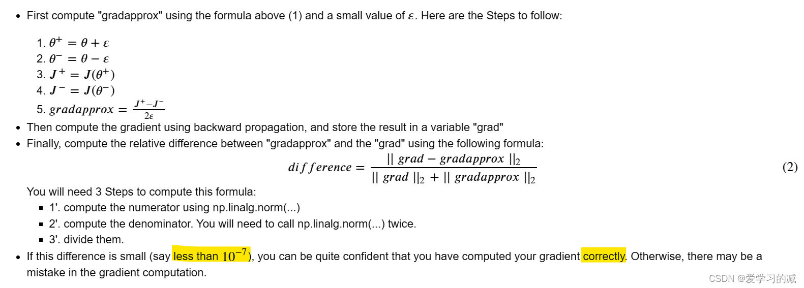
numerator 分子；denominator 分母

def gradient_check(x, theta, epsilon=1e-7, print_msg=False):
"""
实现图1中所示的梯度检查
x——float输入
theta——我们的参数，也是一个float
ε——输入的微小偏移，用公式（1）计算近似梯度
difference——近似梯度和反向传播梯度之间的difference（2） float输出
"""
    # Compute gradapprox using right side of formula (1). epsilon is small enough, you don't need to worry about the limit.

    theta_plus = theta + epsilon                                # Step 1
    theta_minus = theta - epsilon                               # Step 2
    J_plus = forward_propagation(x,theta_plus)                  # Step 3
    J_minus = forward_propagation(x,theta_minus)                # Step 4
    gradapprox = (J_plus + J_minus)/(2 * theta)                 # Step 5
    
    # Check if gradapprox is close enough to the output of backward_propagation()
    grad = backward_propagation(x, theta)

    numerator = np.linalg.norm(gradapprox - grad)                                # Step 1'
    denominator = np.linalg.norm(gradapprox) + np.linalg.norm(grad)              # Step 2'
    difference =  numerator / denominator                                        # Step 3'
 
    if print_msg:
        if difference > 2e-7:
            print ("\033[93m" + "There is a mistake in the backward propagation! difference = " + str(difference) + "\033[0m")
        else:
            print ("\033[92m" + "Your backward propagation works perfectly fine! difference = " + str(difference) + "\033[0m")
    
    return difference

x, theta = 3, 4
difference = gradient_check(x, theta, print_msg=True)

Your backward propagation works perfectly fine! difference = 0.0

5.N维梯度检查

def forward_propagation_n(X, Y, parameters):
"""
实现图3中所示的正向传播（并计算成本）
X——m个例子的训练集
Y——m个示例的标签
parameters--包含参数“W1”、“b1”、“W2”、“b2”、“W3”、”b3“的python字典：
W1——形状（5，4）的权重矩阵
b1——形状（5，1）的偏置矢量
W2——形状（3，5）的权重矩阵
b2——形状（3，1）的偏置矢量
W3——形状（1，3）的权重矩阵
b3——形状（1，1）的偏置矢量
成本——成本函数（m个例子的成本）
cache——具有中间值（Z1、A1、W1、b1、Z2、A2、W2、b2、Z3、A3、W3、b3）的元组
"""
    # retrieve parameters
    m = X.shape[1]    #columns or features
    W1 = parameters["W1"]
    b1 = parameters["b1"]
    W2 = parameters["W2"]
    b2 = parameters["b2"]
    W3 = parameters["W3"]
    b3 = parameters["b3"]

    # LINEAR -> RELU -> LINEAR -> RELU -> LINEAR -> SIGMOID
    Z1 = np.dot(W1, X) + b1
    A1 = relu(Z1)
    Z2 = np.dot(W2, A1) + b2
    A2 = relu(Z2)
    Z3 = np.dot(W3, A2) + b3
    A3 = sigmoid(Z3)

    # Cost
    log_probs = np.multiply(-np.log(A3),Y) + np.multiply(-np.log(1 - A3), 1 - Y)
    cost = 1. / m * np.sum(log_probs)
    
    cache = (Z1, A1, W1, b1, Z2, A2, W2, b2, Z3, A3, W3, b3)
    
    return cost, cache

def backward_propagation_n(X, Y, cache):
"""
实现图2中所示的反向传播
X——输入数据点，形状（输入大小，1）
Y——真“标签”
cache—缓存forward_propation_n（）的输出
梯度——一个字典，包含每个参数、激活和预激活变量的成本梯度
"""
    m = X.shape[1]
    (Z1, A1, W1, b1, Z2, A2, W2, b2, Z3, A3, W3, b3) = cache
    
    dZ3 = A3 - Y
    dW3 = 1. / m * np.dot(dZ3, A2.T)
    db3 = 1. / m * np.sum(dZ3, axis=1, keepdims=True)
    
    dA2 = np.dot(W3.T, dZ3)
    dZ2 = np.multiply(dA2, np.int64(A2 > 0))
    dW2 = 1. / m * np.dot(dZ2, A1.T) * 2
    db2 = 1. / m * np.sum(dZ2, axis=1, keepdims=True)
    
    dA1 = np.dot(W2.T, dZ2)
    dZ1 = np.multiply(dA1, np.int64(A1 > 0))
    dW1 = 1. / m * np.dot(dZ1, X.T)
    db1 = 4. / m * np.sum(dZ1, axis=1, keepdims=True)
    
    gradients = {"dZ3": dZ3, "dW3": dW3, "db3": db3,
                 "dA2": dA2, "dZ2": dZ2, "dW2": dW2, "db2": db2,
                 "dA1": dA1, "dZ1": dZ1, "dW1": dW1, "db1": db1}
    
    return gradients

如果您刚刚实现了这些功能，您可能对它们是否正确工作没有很高的信心。因此，让我们实现梯度检查来帮助验证性能。

梯度检查是如何工作的？

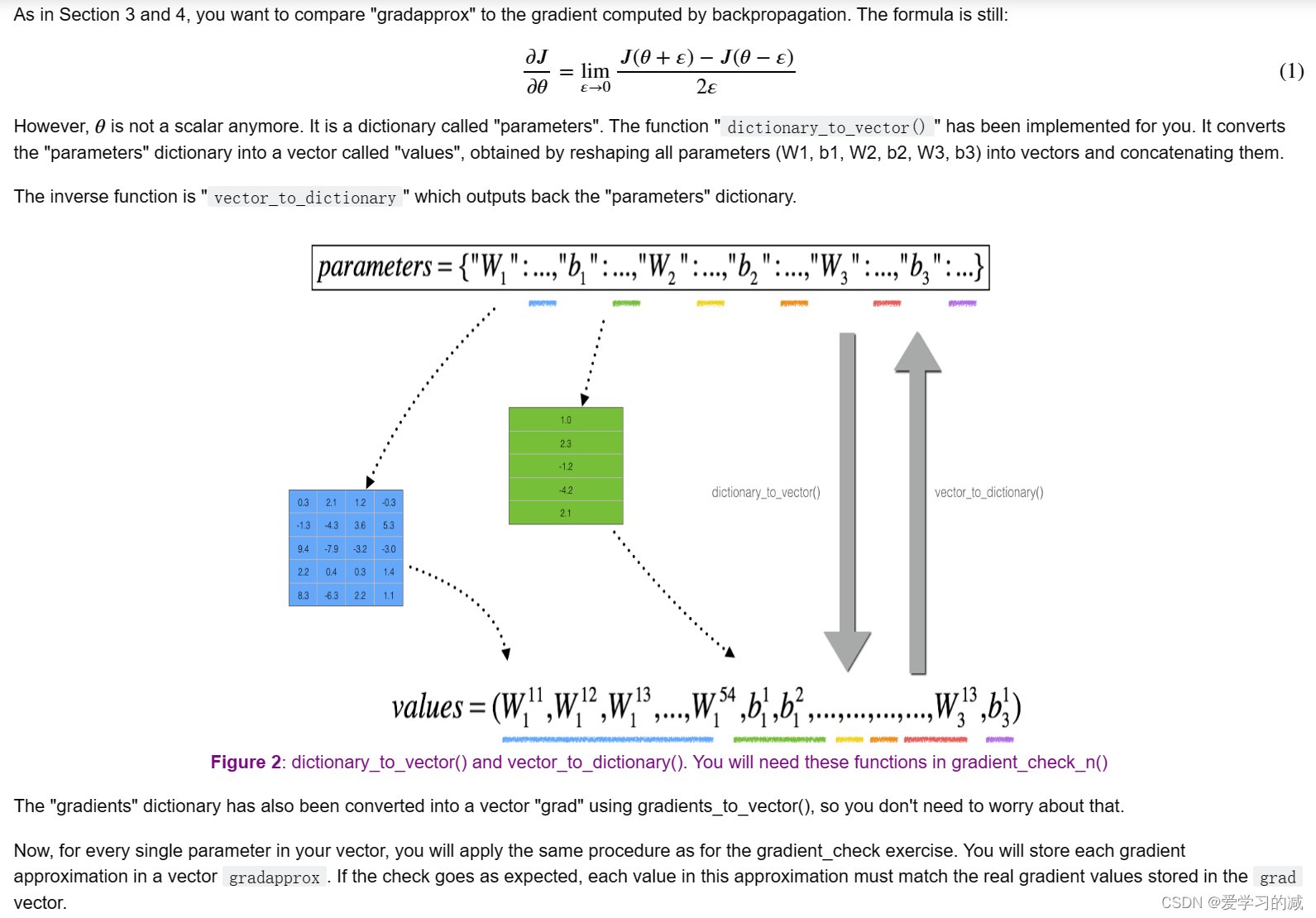
请注意，grad是使用函数gradients_to_vector计算的，该函数使用backward_propation_n函数的梯度输出。

Exercise 4 - gradient_check_n

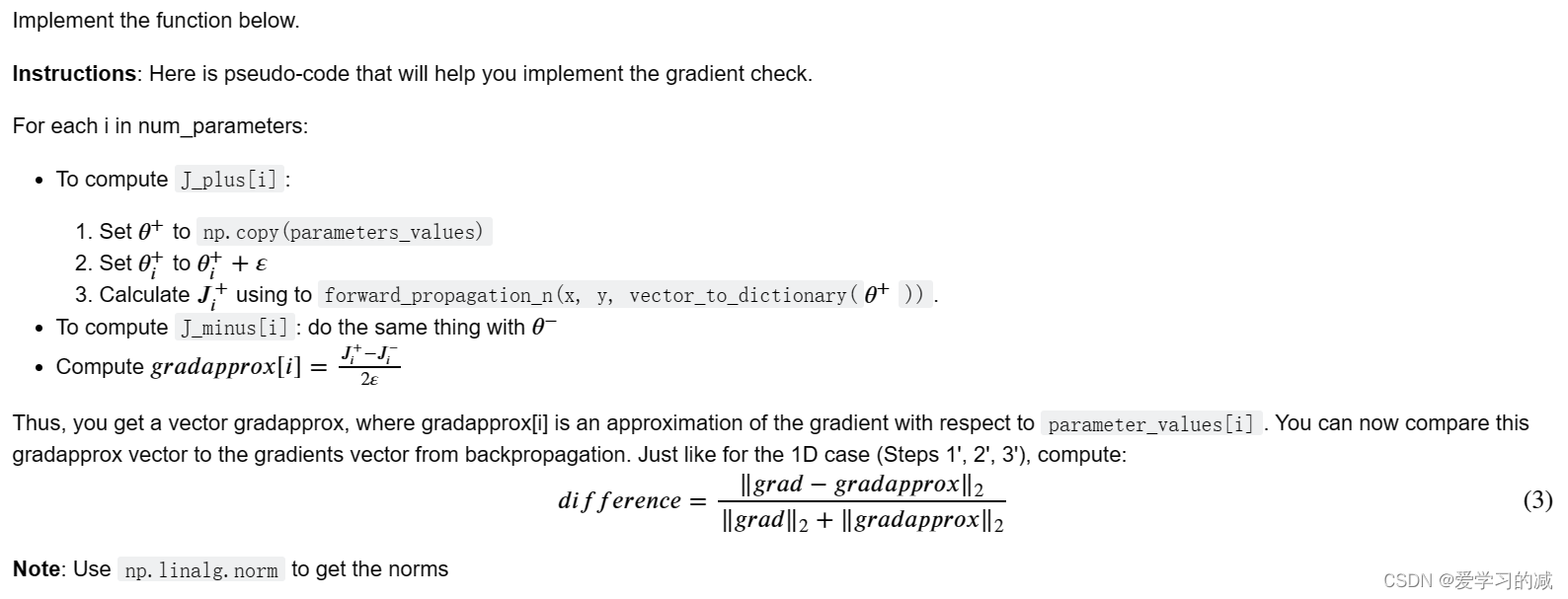
def gradient_check_n(parameters, gradients, X, Y, epsilon=1e-7, print_msg=False):
"""
检查backward_progration_n是否正确计算了forward_progation_n输出的成本梯度
parameters--包含参数“W1”、“b1”、“W2”、“b2”、“W3”、”b3“的python字典
grad——backward_propation_n的输出，包含相对于参数的成本梯度
X——输入数据点，形状（输入大小，示例数）
Y——真“标签”
ε——输入的微小偏移，用公式（1）计算近似梯度
差——近似梯度和反向传播梯度之间的差（2）
"""
def gradient_check_n(parameters, gradients, X, Y, epsilon=1e-7, print_msg=False):
    
    # Set-up variables
    parameters_values, _ = dictionary_to_vector(parameters)
    grad = gradients_to_vector(gradients)
    num_parameters = parameters_values.shape[0]
    J_plus = np.zeros((num_parameters, 1))
    J_minus = np.zeros((num_parameters, 1))
    gradapprox = np.zeros((num_parameters, 1))
    
    # Compute gradapprox
    for i in range(num_parameters):
        
        # Compute J_plus[i]. Inputs: "parameters_values, epsilon". Output = "J_plus[i]".
        thetaplus = np.copy(parameters_values)
        thetaplus[i][0] = thetaplus[i][0] + epsilon
        J_plus[i], _ = forward_propagation_n(X, Y, vector_to_dictionary(thetaplus))
        
        # Compute J_minus[i]. Inputs: "parameters_values, epsilon". Output = "J_minus[i]".
        thetaminus = np.copy(parameters_values)
        thetaminus[i][0] = thetaminus[i][0] - epsilon
        J_minus[i], _ = forward_propagation_n(X, Y, vector_to_dictionary(thetaminus))

        # Compute gradapprox[i]
        gradapprox[i] = (J_plus[i] - J_minus[i]) / (2 * epsilon)

    # Compare gradapprox to backward propagation gradients by computing difference.
    numerator = np.linalg.norm(grad - gradapprox)  # Move this outside the loop
    denominator = np.linalg.norm(grad) + np.linalg.norm(gradapprox)  # Move this outside the loop
    difference = numerator / denominator

    if print_msg:
        if difference > 2e-7:
            print("\033[93m" + "There is a mistake in the backward propagation! difference = " + str(difference) + "\033[0m")
        else:
            print("\033[92m" + "Your backward propagation works perfectly fine! difference = " + str(difference) + "\033[0m")

    return difference

X, Y, parameters = gradient_check_n_test_case()

cost, cache = forward_propagation_n(X, Y, parameters)
gradients = backward_propagation_n(X, Y, cache)
difference = gradient_check_n(parameters, gradients, X, Y, 1e-7, True)
expected_values = [0.2850931567761623, 1.1890913024229996e-07]
assert not(type(difference) == np.ndarray), "You are not using np.linalg.norm for numerator or denominator"
assert np.any(np.isclose(difference, expected_values)), "Wrong value. It is not one of the expected values"

Your backward propagation works perfectly fine! difference = 1.1890913024229996e-07