机器学习——线性模型（二）

【说明】文章内容来自《机器学习——基于sklearn》，用于学习记录。若有争议联系删除。

1、优化方法

线性回归最小二乘法的两种求解方法(即优化方法)分别是正规方程和梯度下降。

1.1?正规方程

????????最小二乘法可以将误差方程转化为有确定解的代数方程组(其方程式数目正好等于未知数的个数)，从而可求解出这些未知数。这个有确定解的代数方程组称为最小二乘法估计的正规方程(normal equation)。
????????正规方程法也称为解析法，采用 Sklearn提供的LinearRegression函数实现。

1.2 正规方法对波士顿房价预测

from sklearn.model_selection import train_test_split
from sklearn.preprocessing import StandardScaler
from sklearn.linear_model import LinearRegression
from sklearn.metrics import mean_squared_error
import pandas as pd
import numpy as np

data_url = "http://lib.stat.cmu.edu/datasets/boston"
raw_df = pd.read_csv(data_url, sep="\s+", skiprows=22, header=None)
data = np.hstack([raw_df.values[::2, :], raw_df.values[1::2, :2]])
target = raw_df.values[1::2, 2]
def linear1():
    x_train, x_test, y_train, y_test = train_test_split(data, target, random_state = 33, test_size = 0.25)
    transfer = StandardScaler()
    x_train = transfer.fit_transform(x_train)
    x_test = transfer.transform(x_test)
    lr = LinearRegression()
    lr.fit(x_train, y_train)
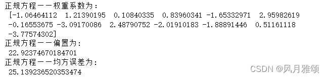
    print('正规方程——权重系数为：\n', lr.coef_)
    print('正规方程——偏置为:\n', lr.intercept_)
    y_predict = lr.predict(x_test)
    error = mean_squared_error(y_test, y_predict)
    print('正规方程——均方误差为:\n', error)
    return None
if __name__ == '__main__':
    linear1()

【运行结果】

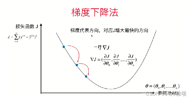
1.3?梯度下降

????????梯度下降(gradient descent)主要用于多元线性回归算法,通过迭代找到目标函数的最小值，或者收敛到最小值。梯度下降法的思想可以类比为下山的过程。当一个人从山顶需要以最快速度下山时,每一刻都以当前所处的位置为基准，寻找从这个位置出发坡度最陡的方向下降。梯度下降法的原理如图所示。

Sklearn提供了SGDRegressor 方法用于梯度下降，格式如下:

SGDRegressor(loss='squared_loss', fit_intercept= True, learning_rate='invscaling')

【参数说明】

• loss= 'squared _loss'：损失函数是最小二乘法。
• fit_intercept：是否计算截距，默认为True.
• learning_rate= 'invscaling'：指定学习率，即下降的步长。

1.4 用梯度下降法对美国波士顿地区房价进行预测。

from sklearn.model_selection import train_test_split
from sklearn.preprocessing import StandardScaler
from sklearn.linear_model import SGDRegressor
from sklearn.metrics import mean_squared_error
import pandas as pd
import numpy as np

data_url = "http://lib.stat.cmu.edu/datasets/boston"
raw_df = pd.read_csv(data_url, sep="\s+", skiprows=22, header=None)
data = np.hstack([raw_df.values[::2, :], raw_df.values[1::2, :2]])
target = raw_df.values[1::2, 2]
def linear2():
    x_train, x_test, y_train, y_test = train_test_split(data, target, random_state = 33, test_size = 0.25)
    transfer = StandardScaler()
    x_train = transfer.fit_transform(x_train)
    x_test = transfer.transform(x_test)
    sgdr = SGDRegressor()
    sgdr.fit(x_train, y_train)
    print('梯度下降——权重系数为：\n', sgdr.coef_)
    print('梯度下降——偏置为:\n', sgdr.intercept_)
    y_predict = sgdr.predict(x_test)
    error = mean_squared_error(y_test, y_predict)
    print('正规方程——均方误差为:\n', error)
    return None
if __name__ == '__main__':
    linear2()

【运行结果】

2、岭回归

2.1 简介

????????岭回归又称为L2正则化。该方法保留全部特征变量，只降低特征变量的系数值，通过弱化参数之间的差异性来避免过拟合。其数学表达式如下:

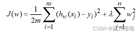
????????岭回归通过对回归系数施加惩罚来解决过拟合问题。具体来说，通过在最小二乘法项后增加L2范数(惩罚项系数)来控制线性模型的复杂程度，从而使模型更加稳健。另一种正则化称为L1正则化，又称为Lasso回归，它通过让参数向量中的许多特征趋近0使它们失去对优化目标的贡献，从此实现目标最小化。
Sklearn 提供了Ridge函数来实现岭回归,格式如下:

sklearn.linear_model.Ridge (alpha=1.0, fit_intercept=True, solver='auto',normalize=False)

【参数说明】

• alpha：正则化力度，即惩罚项系数。
• fit_intercept：是否增加偏置。
• solver：优化器
• normalize：是否进行数据标准化。

属性如下:

• coef_：数组类型，用于权重向量。
• intercept_：截距。当fit _intercept=False时，该属性值为0.0。

方法如下:

• fit(X,y)：训练模型。
• get_params()：获取此估计器的参数。
• predict(X)：使用线性模型进行预测,返回预测值。
• score(X,y)：返回预测性能的得分。
• set_params()：设置此估计器的参数。

2.2 岭回归示例

import numpy as np
import matplotlib.pyplot as plt
from sklearn import linear_model
data=[[83.0, 234.289, 235.6, 159.0, 107.608, 1947., 60.323],
      [88.5, 259.426, 232.5, 145.6, 108.632, 1948., 61.122],
      [88.2, 258.054, 368.2, 161.6, 109.773, 1949., 60.171],
      [89.5, 284.599, 335.1, 165.0, 110.929, 1950., 61.187],
      [96.2, 328.975, 209.9, 309.9, 112.075, 1951., 63.221],
      [98.1, 346.999, 193.2, 359.4, 113.27, 1952., 63.639],
      [99.0, 365.385, 187., 354.7, 115.094, 1953., 64.989],
      [100.0, 363.112, 357.8, 335.0, 116.219, 1954., 63.761],
      [101.2, 397.469, 290.4, 304.8, 117.388, 1955., 66.019],
      [104.6, 419.18, 282.2, 285.7, 118.734, 1956., 67.857],
      [108.4, 442.769, 293.6, 279.8, 120.445, 1957., 68.169],
      [110.8, 444.546, 468.1, 263.7, 121.95, 1958., 66.513],
      [112.6, 482.704, 381.3, 255.2, 123.366, 1959., 68.655],
      [114.2, 502.601, 393.1, 251.4, 125.368, 1960., 69.564],
      [115.7, 518.173, 480.6, 257.2, 127.852, 1961., 69.331],
      [116.9, 554.894, 400.7, 282.7, 130.081, 1962., 70.5511]]
data = np.array(data)
X_data = data[:,1:]
y_data = data[:,0]
print(X_data)
print(y_data)
#岭回归模型
alpha = 0.5
model = linear_model.Ridge(alpha)
model.fit(X_data, y_data)
#返回模型的估计系数
print(model.coef_)
#评分
model.score(X_data,y_data)
#创建模型,开始训练,生成50个alpha系数
alphas=np.linspace(0.001, 1, 50)
#RidgeCV表示岭回归交叉检验,类似于留一交叉验证法
#它在训练时保留一个样本,用这个样本进行测试
cv_model = linear_model.RidgeCV(alphas, store_cv_values = True)
cv_model.fit(X_data, y_data)
#最佳的alpha
best_alpha = cv_model.alpha_
print(best_alpha)
#交叉验证的结果
print(cv_model.cv_values_)
print(cv_model.cv_values_.shape)
#结果中(16,50)指数据被拆分为16份,做了16次训练和测试，每次训练集使用15份数据
#测试集使用1份数据，每次使用50个alpha值进行训练
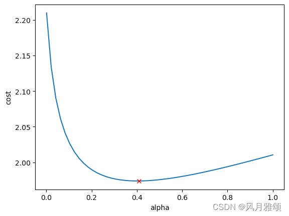
#针对所有alpha值计算出的损失值
plt.plot(alphas, cv_model.cv_values_.mean(axis=0))
#最佳点
min_cost=min(cv_model.cv_values_.mean(axis=0))
plt.plot(best_alpha, min_cost, 'rx')
plt.xlabel('alpha')
plt.ylabel('cost')
plt.show()

【运行结果】

2.3 alpha参数

????????岭回归的alpha参数作为惩罚项的系数，对应于其他线性模型(如逻辑回归LinearSVC)中的C参数。下面通过调整alpha参数值分析线性模型的拟合程度。

from sklearn.model_selection import train_test_split
from sklearn.datasets import load_diabetes
x, y = load_diabetes().data, load_diabetes().target
x_train, x_test, y_train, y_test = train_test_split(x, y, random_state = 8)
from sklearn.linear_model import Ridge
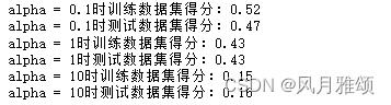
ridge01 = Ridge(alpha = 0.1).fit(x_train, y_train)
print('alpha = 0.1时训练数据集得分：{:.2f}'.format(ridge01.score(x_train, y_train)))
print('alpha = 0.1时测试数据集得分：{:.2f}'.format(ridge01.score(x_test, y_test)))
ridge1 = Ridge(alpha = 1).fit(x_train, y_train)
print('alpha = 1时训练数据集得分：{:.2f}'.format(ridge1.score(x_train, y_train)))
print('alpha = 1时测试数据集得分：{:.2f}'.format(ridge1.score(x_test, y_test)))
ridge10 = Ridge(alpha = 10).fit(x_train, y_train)
print('alpha = 10时训练数据集得分：{:.2f}'.format(ridge10.score(x_train, y_train)))
print('alpha = 10时测试数据集得分：{:.2f}'.format(ridge10.score(x_test, y_test)))

【运行结果】

3、案例

3.1 线性回归和岭回归用于糖尿病预测

#线性回归
from sklearn.model_selection import train_test_split
from sklearn.linear_model import LinearRegression
from sklearn.datasets import load_diabetes
x, y = load_diabetes().data, load_diabetes().target
x_train, x_test, y_train, y_test = train_test_split(x, y, random_state = 8)
lr = LinearRegression().fit(x_train, y_train)
print('训练数据集得分：{:.2f}'.format(lr.score(x_train, y_train)))
print('测试数据集得分：{:.2f}'.format(lr.score(x_test, y_test)))

#岭回归
from sklearn.model_selection import train_test_split
from sklearn.linear_model import Ridge
from sklearn.datasets import load_diabetes
x, y = load_diabetes().data, load_diabetes().target
x_train, x_test, y_train, y_test = train_test_split(x, y, random_state = 8)
ridge = Ridge().fit(x_train, y_train)
print('训练数据集得分：{:.2f}'.format(ridge.score(x_train, y_train)))
print('测试数据集得分：{:.2f}'.format(ridge.score(x_test, y_test)))

3.2 最小二乘法和岭回归用于波士顿房价预测

#最小二乘法和领回归应用波士顿
from sklearn import datasets
import numpy as np
import matplotlib.pyplot as plt
import pandas as pd
data_url = "http://lib.stat.cmu.edu/datasets/boston"
raw_df = pd.read_csv(data_url, sep="\s+", skiprows=22, header=None)
data = np.hstack([raw_df.values[::2, :], raw_df.values[1::2, :2]])
target = raw_df.values[1::2, 2]
x = data
y = target
sampleRatio=0.5  #划分训练集和测试集,各用一半数据
m=len(x)
sampleBoundary=int(m* sampleRatio)
myshuffle=list(range(m))  #range返回序列
np.random.shuffle(myshuffle)  # shuffle将序列内的元素全部随机排序
#分别取出训练集和测试集的数据
train_fea=x[myshuffle[sampleBoundary:]]#前一半数据作为训练集
train_tar=y[myshuffle[sampleBoundary:]]
test_fea=x[myshuffle[:sampleBoundary]]#后一半数据作为测试集
test_tar=y[myshuffle[:sampleBoundary]]
#使用最小二乘线性回归进行拟合
from sklearn import linear_model
#最小二乘线性
lr=linear_model.LinearRegression()
#拟合
lr.fit(train_fea, train_tar)
#得到预测值集合
y=lr.predict(test_fea)

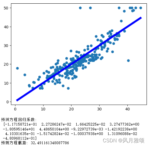
plt.scatter(y,test_tar)   #画出散点图,横轴是预测值,纵轴是真实值
                    #将实际房价数据与预测数据对比，接近中间直钱的数据表示预测准确
plt.plot([y.min(),y.max()],[y.min(),y.max()],'b',lw = 5)
                        #直线的起点为(y,min()，y.min()),终点是(y.max(),y.max())
plt.show()
coef=lr.coef_
intercept = lr.intercept_
print("预洲方程回归系数:\n",coef)
print("预测方程截距:",intercept)

【运行结果】

import numpy as np
import matplotlib.pyplot as plt
import pandas as pd
from sklearn.model_selection import train_test_split
from sklearn.preprocessing import StandardScaler
from sklearn.linear_model import Ridge
from sklearn.metrics import mean_squared_error
data_url = "http://lib.stat.cmu.edu/datasets/boston"
raw_df = pd.read_csv(data_url, sep="\s+", skiprows=22, header=None)
data = np.hstack([raw_df.values[::2, :], raw_df.values[1::2, :2]])
target = raw_df.values[1::2, 2]
def linear3():
    x_train, x_test, y_train, y_test = train_test_split(data, target, random_state = 33, test_size = 0.25)
    transfer = StandardScaler()
    #分别对训练和测试数据的特征以及目标值进行标准化处理
    x_train = transfer.fit_transform(x_train)
    x_test = transfer.transform(x_test)
    #预估器选择岭回归
    estimator = Ridge()
    estimator.fit(x_train, y_train)
    #得出模型，输出回归系数和偏置
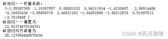
    print('岭回归——权重系数：\n',estimator.coef_)
    print('岭回归——偏置为:\n',estimator.intercept_)
    y_predict = estimator.predict(x_test)
    error = mean_squared_error(y_test, y_predict)
    print('岭回归均方误差为:\n',error)
    return None
if __name__ == '__main__':
    linear3()

【运行结果】

3.3 逻辑回归应用于鸢尾花分类

from sklearn.decomposition import PCA
from sklearn.datasets import load_iris
from sklearn.linear_model import LogisticRegression
import matplotlib.pyplot as plt
import numpy as np
plt.rcParams['font.sans-serif'] = ['SimHei']
plt.rcParams['font.family'] = 'sans-serif'
plt.rcParams['axes.unicode_minus'] = False
iris = load_iris()
iris_data = iris.data
iris_target = iris.target
print(iris_data.shape)
pca = PCA(n_components = 2)#特征降维
x = pca.fit_transform(iris_data)
print(x.shape)
f = plt.figure()
ax = f.add_subplot(111)
ax.plot(x[:,0][iris_target == 0],x[:, 1][iris_target == 0], 'bo')
ax.scatter(x[:,0][iris_target == 1], x[:, 1][iris_target == 1], c = 'r')
ax.scatter(x[:, 0][iris_target == 2], x[:, 1][iris_target == 2], c = 'y')
ax.set_title('数据分布图')
plt.show ()
clf=LogisticRegression(multi_class = 'ovr', solver = 'lbfgs', class_weight={0:1, 1:1, 2:1})
clf.fit(x, iris_target)
score = clf.score (x, iris_target)
x0min, x0max = x[:, 0].min(), x[:, 0].max()
x1min, x1max = x[:, 1].min(), x[:, 1].max ()
h=0.05
xx, yy = np.meshgrid(np.arange (x0min - 1, x0max + 1, h), np.arange(x1min -1, x1max+1, h))
x_ = xx.reshape([xx.shape[0] * xx.shape[1], 1])
y_ = yy.reshape([yy.shape[0] * yy.shape[1], 1])
test_x = np.c_[x_, y_]
test_predict = clf.predict(test_x)
z = test_predict.reshape (xx.shape)
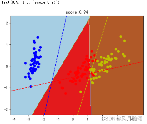
plt.contourf(xx, yy, z, cmap = plt.cm.Paired)
plt.axis('tight')
colors = 'bry'
for i, color in zip(clf.classes_, colors):
         
    idx = np.where(iris_target == i)
    plt.scatter(x[idx, 0], x[idx, 1], c = color, cmap = plt.cm.Paired)
xmin,xmax = plt.xlim()
coef = clf.coef_
intercept = clf.intercept_
def line(c, x0):
    return (-coef[c,0]*x0 - intercept[c]) /coef[c, 1]
for i, color in zip(clf.classes_, colors):
    plt.plot([xmin, xmax], [line(i, xmin), line(i, xmax)], color = color, linestyle ='--')
plt.title("score:{0}".format(score))

【运行结果】

? ? ? ??