【AI核心能力】第5讲 机器学习三

第5讲 机器学习三

How does this world run?

• Functionality
• Probability
• Imitating
• Diversion
• Split spaces
• Collective intelligences

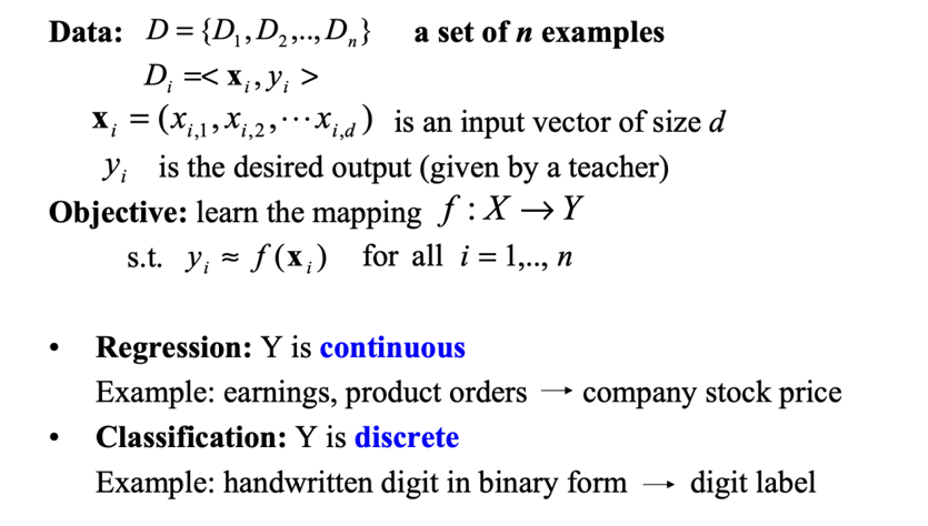
Supervised Learning

KNN

KNN的思路其实很简单

要解决这个回归问题，KNN的思路就是取距离x很近的几个点的y值求均值

要解决这个分类问题，KNN的思路就是取距离该点最近的点统计个数，看X多还是O多

(xs, ys) = sort((xi, yi) for (xi, yi) in D, key = distance(xi, x))[:k]

• if regression
  $$\hat{y}=np.mean(y_s)$$

• if classification
  $$\hat{y}=Counter(y_s).most?common()$$

最好的深度学习模型所达到的效果就是经过仔细（sophisticated）调参过的KNN

KNN的

• 优点

  • 容易实现、容易理解
  • 模型调整容易，可以方便得改变k的数量，或者给不同距离的k进行加权
  • 适合解决各种复杂问题（分类、回归、高纬、低纬、复杂关系、简单关系）

• 缺点

  • 运行时间久

    • 问：KNN的时间复杂度是多少？

    • 如果是 2.7Ghz 英特尔i7处理器，训练数据有1亿个数据是300维，定义的k=11，则预测100个实例需要大约多久？

    • A. 几毫秒； B. 几秒 ； C. 几分钟 ；D. 几个小时 ；E. 几天
      $$\begin{gathered} 10^8?logk?300?100\approx 10^{13} \\ 2.7GHz=1s运行10^9次 \\ 需运行10^{4}s\approx 2.78h \end{gathered}$$

  • 容易被异常值影响

  • 所需空间大

  • 高维空间的距离区分度不大

Eager Learning & Lazy Learning

KNN属于lazy learning因为它没有显示的学习过程，而是直接根据已有数据进行决策。

贝叶斯分类 Bayesian Classfier

对于某种商品，根据以往购买的数据，在任意投放广告，未进行特点渠道优化的时候，点击广告到购买商品的比率为7%， 自然形成的用户中，本科及以上学历的用户占15%，本科以下学历占85%；现在有一笔广告预算，本科及以上学历渠道的获客成本市场100元每人，本科以下人群投放广告的成本是70元每人。问，该广告该投放到本科及以上学历专门的人群还是本科以下人群？(本科及以上学历占总国人的比例约为5%，2016年国家统计局数据)

贝叶斯公式
$$\begin{gathered} Pr(购买\mid 本科及以上)=Pr(本科及以上\mid 购买)?Pr(购买)/Pr(本科及以上)=15\%?7\%/5\%=21\% \\ Pr(购买\mid 本科以下)=Pr(本科以下\mid 购买)?Pr(购买)/Pr(本科以下)=85\%?7\%/95\%=6.26\% \\ 本科及以上每个人的广告成本为100/21\%=476元 \\ 本科以下每个人的广告成本为70/6.26\%=1118元 \\ 产品卖2千元，则花费100万广告费，只投放给本科以及上人群，则公司可以收入100万/476?2千=420万 \\ 产品卖2千元，则花费100万广告费，人群，则公司可以收入100万/1118?2千=178万 \end{gathered}$$

朴素贝叶斯分类器 Naive Bayesian Classfier

$$\begin{array}{rl}p\left(C_k,x_1,\dots ,x_n\right)& =p\left(x_1,\dots ,x_n,C_k\right)\\ & =p\left(x_1\mid x_2,\dots ,x_n,C_k\right)p\left(x_2,\dots ,x_n,C_k\right)\\ & =p\left(x_1\mid x_2,\dots ,x_n,C_k\right)p\left(x_2\mid x_3,\dots ,x_n,C_k\right)p\left(x_3,\dots ,x_n,C_k\right)\\ & =\dots \\ & =p\left(x_1\mid x_2,\dots ,x_n,C_k\right)p\left(x_2\mid x_3,\dots ,x_n,C_k\right)\dots p\left(x_{n?1}\mid x_n,C_k\right)p\left(x_n\mid C_k\right)p\left(C_k\right)\end{array}$$

带入一个识别垃圾邮件的情景
$$\begin{array}{rl}p\left(spam|text\right)& =p\left(spam\mid w_1,w_2,\dots ,w_n\right)\\ & =\frac{p(w_1,w_2,\dots ,w_n\mid spam)p(spam)}{p(w_1,w_2,\dots ,w_n)}\\ & =\frac{p(w_1,w_2,\dots ,w_n?spam)}{p(w_1,w_2,\dots ,w_n)}\\ & =\frac{p\left(w_1\mid w_2,w_3,\dots ,w_n?spam\right)p\left(w_2,w_3,\dots ,w_n?spam\right)}{p(w_1,w_2,\dots ,w_n)}\\ & =\frac{p\left(w_1\mid w_2,w_3,\dots ,w_n?spam\right)p\left(w_2\mid w_3,w_4,\dots ,w_n?spam\right)p\left(w_3,w_4,\dots ,w_n?spam\right)}{p(w_1,w_2,\dots ,w_n)}\\ & =\dots \\ & =\frac{p\left(w_1\mid w_2,w_3,\dots ,w_n?spam\right)p\left(w_2\mid w_3,w_4,\dots ,w_n?spam\right)\dots p(w_n\mid spam)p(spam)}{p(w_1,w_2,\dots ,w_n)}\\ & \approx \prod _i^{n}p(w_i\mid spam)p(spam)\end{array}$$
带入一个预测车辆是否被偷的情景

我们要计算p(Steal)
$$\begin{array}{rl}p(Steal)& :p(Yellow\mid Stolen)p(Sports\mid Stolen)p(Imported\mid Stolen)p(Stolen)\\ & =\frac{2}{5}\frac{4}{5}\frac{3}{5}\frac{1}{2}=\frac{24}{250}\\ & :p(Yellow\mid \overline{Stolen})p(Sports\mid \overline{Stolen})p(Imported\mid \overline{Stolen})p(\overline{Stolen})\\ & =\frac{3}{5}\frac{2}{5}\frac{2}{5}\frac{1}{2}=\frac{12}{250}\end{array}$$
这意味着购买一辆黄色进口跑车，被偷的概率是不被偷的2倍

高斯贝叶斯分类器 Gaussian Bayesian Classifier

When dealing with continuous data, a typical assumption is that the continuous values associated with each class are distributed according to a Gaussian distribution. For example, suppose the training data contains a continuous attribute x

$$p(x=v\mid C_k)=\frac{1}{\sqrt{2\pi {\sigma }_k^2}}{e}^{?\frac{(v?{\mu }_k{)}^2}{2{\sigma }_k^2}}$$

用于处理连续值的问题。

贝叶斯分类器的

• 优点
  • Easy to implement
  • It is highly scalable with the number of predictors and data points
  • It is fast and can be used to make real-time predictions
• 缺点
  • It is not sensitive to irrelevant features ——容易陷入历史局限性

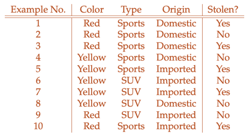
支持向量机 Support Vector Machine

形象的说，我们要找到一条直线使其分割两部分点，点到直线的距离为长度的向量 会来回拨动这条直线，使其最终固定在一个位置。这些向量就被叫做支撑向量。

import numpy as np

label_a = np.random.normal(6, 2, size=(50, 2))
label_b = np.random.normal(-6, 2, size=(50, 2))

import matplotlib.pyplot as plt

plt.scatter(*zip(*label_a))
plt.scatter(*zip(*label_b))

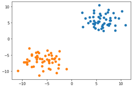
我们通过控制直线在大于0和小于0处的正负值来分割两部分点

def f(x, k, b):
    return k * x - b
    
k_and_b = []

for i in range(100):
    k, b = (np.random.random(size=(1, 2)) * 10 - 5)[0]

    label_a_x = label_a[:, 0]
    label_b_x = label_b[:, 0]

    if np.max(f(label_a_x, k, b)) <= -1 and np.min(f(label_b_x, k, b)) >= 1:
        k_and_b.append((k, b))
        
plt.scatter(*zip(*label_a))
plt.scatter(*zip(*label_b))

for k, b in k_and_b:
    x = np.concatenate((label_a, label_b))
    plt.plot(x, f(x, k, b))

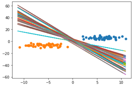
但这样的结果显然不够好，我们要做的是对于
$$y_i(w?x_i?b)>?$$
构造一个损失函数，使得我们获得最大的两点间最近距离
$$\frac{2}{|W|}$$
之所以将函数写成如上形式，是因为我们希望对于一部分点有：w * xi - b > 1；对于另外一部分点有：w * xi - b < -1。因此，我们将label作为 yi，就可以表示成一个式子写入Loss函数。

HingeLoss

我们如下构造这个Loss函数
$$loss=max(0,1?y_i?(w?x_i?b))$$
为了更快地找到最小的 |w|，我们要加上一个regularization
$$loss=max(0,1?y_i?(w?x_i?b))+\lambda |w{|}^2$$
核函数 kernel function

当然，很多时候我们遇到的问题是没法用线性函数进行切割，此时需要用变换函数对数据进行变换，这样的函数被称为核函数。

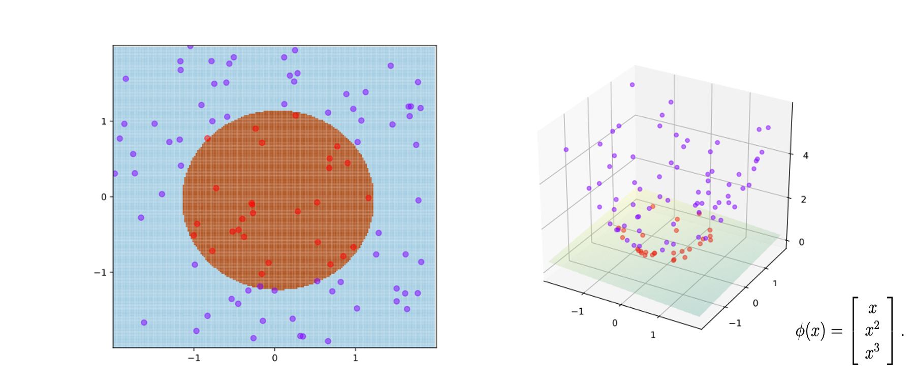
SVM曾经是和深度学习一样的热门研究领域，原因就在于人们不断提出新的核函数，使得在低维空间没法切割的数据在高位空间变得可切割。

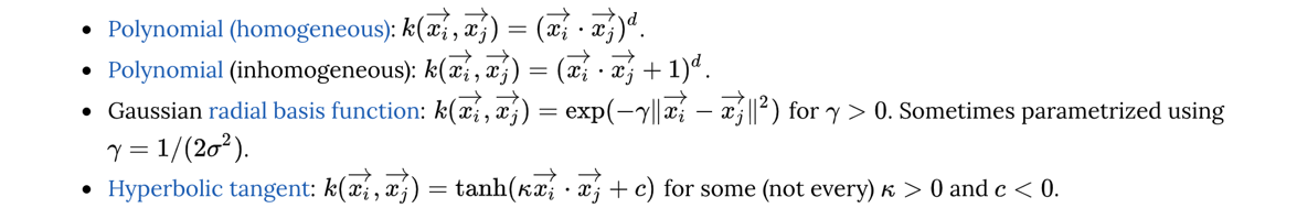
下面是一些科学家提出的常用核函数

SVM为什么能找到最优的线性分割点（最优直线）？

• w求最小，小于-1大于1求最小w

SVM的损失函数是什么

• HingeLoss

SVM核函数的作用是什么

• 变换函数

SVM的

• 优点
  • 当维度比较少的时候计算得比较快
  • 能解决不平衡的问题——可以根据数据的重要性增加或减小权重（比如将上面的代码中的-1改成-4）
• 缺点
  • 维度较多的时候找不到合适的核函数

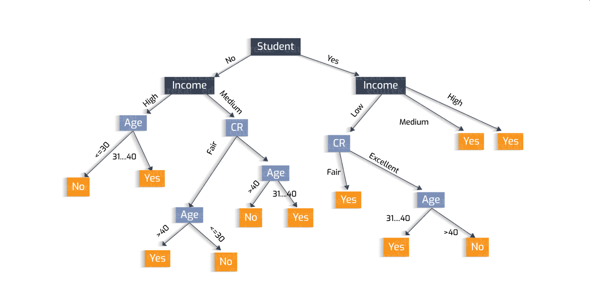
决策树 Decision Tree

决策树模型，让计算机自动构建逐层的 if-else 模型

CART Algorithm:

Classification And Regression Tree Algorithm

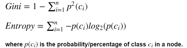
这个树的算法核心就是要衡量一个指标，这个指标一般是基尼系数或者熵（都是用来表示杂乱程度 的）

import numpy as np
from collections import Counter

def pr(e, es):
    return Counter(es)[e] / len(es)
    
def gini(elements):
    return 1 - np.sum(pr(e, elements)**2 for e in set(elements))

def entropy(elements):
    return -np.sum(pr(e, elements)*np.log2(pr(e, elements)) for e in set(elements))

features_1 = ['R', 'R', 'Y', 'Y']
features_2 = ['R', 'R', 'R', 'Y']
features_3 = ['R', 'R', 'R', 'R']

gini(features_1)
### Output:
### 0.5
gini(features_1)
### Output:
### 0.375
gini(features_1)
### Output:
### 0.0
entropy(features_1)
### Output:
### 1.0
entropy(features_1)
### Output:
### 0.8112781244591328
entropy(features_1)
### Output:
### -0.0

举个例子，我们按照某种特征对Label进行分类，希望分出来的数据混乱程度最小（接近0）

import pandas as pd

item_scales = {
    'gender':['F', 'F', 'F', 'F', 'M', 'M', 'M'],
    'income':['20', '10', '20', '20', '20', '20', '10'],
    'family_number':[1, 1, 2, 1, 1, 1, 2],
    'bought':[1, 1, 1, 0, 0, 0, 1]
}

dataset = pd.DataFrame.from_dict(item_scales)

target = 'bought'

print(dataset[dataset['gender'] == 'F'][target].tolist(), dataset[dataset['gender'] == 'M'][target].tolist())
gini(dataset[dataset['gender'] == 'F'][target].tolist()) + gini(dataset[dataset['gender'] == 'M'][target].tolist())
### Output:
### [1, 1, 1, 0] [0, 0, 1]
### 0.8194444444444444

print(dataset[dataset['income'] == '20'][target].tolist(), dataset[dataset['income'] == '10'][target].tolist())
gini(dataset[dataset['income'] == '20'][target].tolist()) + gini(dataset[dataset['income'] == '10'][target].tolist())
### Output:
### [1, 1, 0, 0, 0] [1, 1]
### 0.48

这就是决策树构建的原理，Loss函数如下：将m分成左右两类，各自比例*各自基尼
$$Loss=m_{left}/m?G_{left}+m_{right}/m?G_{right}$$

决策树可以做回归吗

回归问题的本质在于得到一个数（实数或向量）
$$J\left(k,t_k\right)=\frac{m_{\text{left?}}}{m}{\mathrm{MSE}}_{\text{left?}}+\frac{m_{\text{right?}}}{m}{\mathrm{MSE}}_{\text{right?}}\text{?where?}\{\begin{array}{l}{\mathrm{MSE}}_{\text{node?}}={\sum }_{i\in \text{?node?}}{\left({\hat{y}}_{\text{node?}}?y^{(i)}\right)}^2\\ {\hat{y}}_{\text{node?}}=\frac{1}{m_{\text{node?}}}{\sum }_{i\in \text{?node?}}{y}^{(i)}\end{array}$$
比如现在有几个y：[9.1, 3.2, 5.3, 8.9, 4.3]，那么通过上面的Loss函数就可以将 [3.2, 5.3, 4.3] 分在一块，将 [9.1, 8.9] 分在一块，从而进行回归。

决策树的

• 优点
  • Clear to explain
  • Could select salient features——显著特征（最能区分的那些特征）会在决策树的上层，决策树可以找出这些重要的特征，然后再送到深度学习模型中去做更精密的拟合
• 缺点
  • So sensitive——异常值可能会出现在树的上层，容易过拟合
  • Fit ability is limited——拟合能力有限，处理高维数据必须要构造很深的一棵树；或者特征比较均匀找不到区分点

我们使用决策树做一个回归，看看它是怎么帮助我们找到显著特征的

from sklearn.datasets import load_boston

boston = load_boston()
X = boston.data
y = boston.target

from sklearn.tree import DecisionTreeRegressor

tree_clf = DecisionTreeRegressor()
tree_clf.fit(X, y)
### Output:
### DecisionTreeRegressor(criterion='mse', max_depth=None, max_features=None,
###                       max_leaf_nodes=None, min_impurity_decrease=0.0,
###                       min_impurity_split=None, min_samples_leaf=1,
###                       min_samples_split=2, min_weight_fraction_leaf=0.0,
###                       presort=False, random_state=None, splitter='best')

安装合适的软件可以将决策树区分结果画出来，这里我们直接看内容

from sklearn.tree import export_graphviz

export_graphviz(tree_clf, out_file='boston.dot', feature_names=boston.feature_names, rounded=True, filled=True)

for line in open('boston.dot'):
    print(line)
### Output:
### digraph Tree {
### node [shape=box, style="filled, rounded", color="black", fontname=helvetica] ;
### edge [fontname=helvetica] ;

### 0 [label="RM <= 6.941\nmse = 84.42\nsamples = 506\nvalue = 22.533", fillcolor="#f5ceb2"] ;

### 1 [label="LSTAT <= 14.4\nmse = 40.273\nsamples = 430\nvalue = 19.934", fillcolor="#f6d5bd"] ;
### 0 -> 1 [labeldistance=2.5, labelangle=45, headlabel="True"] ;

### 2 [label="DIS <= 1.385\nmse = 26.009\nsamples = 255\nvalue = 23.35", fillcolor="#f4ccae"] ;
### 1 -> 2 ;

### 3 [label="CRIM <= 10.592\nmse = 78.146\nsamples = 5\nvalue = 45.58", fillcolor="#e88d4c"] ;
### 2 -> 3 ;

### 4 [label="mse = 0.0\nsamples = 4\nvalue = 50.0", fillcolor="#e58139"] ;
### 3 -> 4 ;

### 5 [label="mse = -0.0\nsamples = 1\nvalue = 27.9", fillcolor="#f2bf9a"] ;
### 3 -> 5 ;

### 6 [label="RM <= 6.543\nmse = 14.885\nsamples = 250\nvalue = 22.905", fillcolor="#f5cdb0"] ;
### 2 -> 6 ;

### 7 [label="LSTAT <= 7.57\nmse = 8.39\nsamples = 195\nvalue = 21.63", fillcolor="#f5d0b6"] ;
### 6 -> 7 ;

### 8 [label="TAX <= 222.5\nmse = 3.015\nsamples = 43\nvalue = 23.97", fillcolor="#f4caac"] ;

### ...

### 938 [label="mse = -0.0\nsamples = 1\nvalue = 21.9", fillcolor="#f5d0b5"] ;
### 892 -> 938 ;
### }

sorted({n:w for n,w in zip(boston.feature_names, tree_clf.feature_importances_)}.items(), key=lambda x:x[1], reverse=True)
### Output:
### [('RM', 0.5907091048839664),
###  ('LSTAT', 0.1963431191613278),
###  ('DIS', 0.07280894664958623),
###  ('CRIM', 0.07011069274201277),
###  ('NOX', 0.026601986615508035),
###  ('TAX', 0.012019253220591294),
###  ('AGE', 0.01068973495782809),
###  ('PTRATIO', 0.007601724863367392),
###  ('B', 0.00708663404275688),
###  ('INDUS', 0.003671588474370431),
###  ('CHAS', 0.0010479321144977688),
###  ('RAD', 0.0006709656440991935),
###  ('ZN', 0.0006383166300875832)]

可以看到，我们对特征重要程度进行排序后就找到了决策树上层的几个特征，也就是显著特征。有了显著特征，如果现有模型的准确率不高，那么我们就可以选择排名前几的特征喂给贝叶斯或者KNN之类的模型。

维度降低意味着数据量变小了，也正因此，可以使用决策树帮助其他模型进行学习。

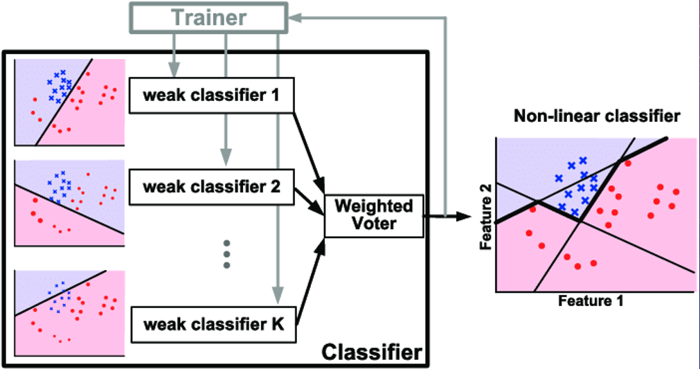
集成学习 Ensemble Learning

我们把在机器学习过程中用到多个模型的这种学习方式叫作集成学习（ensemble learning），本质上就是分开学习、集中投票，一般使用方式如下

from sklearn.ensemble import RandomForestClassifier
from sklearn.ensemble import VotingClassifier
from sklearn.linear_model import LogisticRegression
from sklearn.svm import SVC

log_clf = LogisticRegression()
rnd_clf = RandomForestClassifier()
svm_clf = SVC()

voting_clf = VotingClassifeer(
    		estimators=[('lr', log_clf), ('rf', rnd_clf), ('svc', svm_clf)],
    		voting='hard'
)
voting_clf.fit(X_train, y_train)

Bagging和Boosting都是集成学习的技术，旨在通过将多个弱学习器组合在一起来构建一个强大的预测模型。它们的主要思想和一些异同点如下：

Bagging（自助采样聚合）：

• 思想： Bagging使用自助采样的方法，从训练数据集中有放回地随机抽取多个子集，然后在每个子集上训练弱学习器，最后将这些弱学习器的预测进行平均或投票来进行集成。
• 过程： 由于采用了自助采样，每个子集可能会包含重复样本，这样会有一些样本被多次采样，而一些样本可能被忽略。
• 集成： 最终的预测通常是将弱学习器的预测进行平均（对回归问题）或投票（对分类问题）得到。

Boosting（提升）：

• 思想： Boosting是一种逐步改进的方法，它通过顺序训练多个弱学习器，并在每一轮训练中，对之前模型预测不准确的样本加以更多关注，从而逐渐提升整体性能。
• 过程： 在每一轮训练中，模型会赋予错误分类样本更高的权重，以便后续弱学习器能够更好地拟合这些难以分类的样本。
• 集成： 最终的预测是通过将所有弱学习器的预测进行加权求和得到，权重由每个弱学习器的表现决定。

异同点：

1. 样本选择： Boosting在每一轮迭代中都会调整样本权重，更多地关注之前分类错误的样本；而Bagging使用自助采样，每个子集之间的样本是独立采样的。
2. 弱学习器关系： Boosting的弱学习器之间存在依赖关系，每个弱学习器都在尝试修正之前学习器的错误；Bagging的弱学习器是独立的，彼此之间没有依赖关系。
3. 权重调整： Boosting通过逐步调整样本权重来改善模型的表现；Bagging不涉及样本权重调整，所有子集的样本在模型训练中具有相同的权重。

下面介绍两种集成思想的实际应用

随机森林 Random Forest —— Bagging

因为决策树经常会有过拟合的情况出现，所以有些人通过随机抽取一些特征数据来预测，然后将多个决策树模型合在一起（集体智慧），往往会有更好的效果。

The Single Model Performance

from sklearn.datasets import load_boston
import pandas as pd

boston = load_boston()
x, y = boston['data'], boston['target']

dataframe = pd.DataFrame(x)
dataframe.columns = boston['feature_names']

from sklearn.model_selection import train_test_split

(X_train, X_test, y_train, y_test) = train_test_split(x, y, test_size=0.3)

from sklearn.tree import DecisionTreeRegressor

regressor = DecisionTreeRegressor()
regressor.fit(X_train, y_train)
### Output:
### DecisionTreeRegressor(criterion='mse', max_depth=None, max_features=None,
###                       max_leaf_nodes=None, min_impurity_decrease=0.0,
###                       min_impurity_split=None, min_samples_leaf=1,
###                       min_samples_split=2, min_weight_fraction_leaf=0.0,
###                       presort=False, random_state=None, splitter='best')

regressor.score(X_train, y_train)
### Output:
### 1.0
regressor.score(X_test, y_test)
### Output:
### 0.6343814965530834

The Power of Multi-Model

import random

def random_select(dataframe, y, drop_num=4):
    columns = random.sample(list(dataframe.columns), k=len(dataframe.columns)  - drop_num)
    indices = np.random.choice(range(len(dataframe)), size=len(dataframe), replace=True)
    return dataframe.iloc[indices][columns], y[indices]
    
(train_X, test_X, train_y, test_y) = train_test_split(dataframe, y, test_size=0.3)
split_data = (train_X, test_X, train_y, test_y)

def random_tree(train_X, test_X, train_y, test_y, drop_num=4):
    train_sample, bagging_y = random_select(train_X, train_y, drop_num=drop_num)
    regressor = DecisionTreeRegressor()
    regressor.fit(train_sample, bagging_y)

    train_score = regressor.score(train_sample, bagging_y)
    test_score = regressor.score(test_X[train_sample.columns], test_y)
    print('training score and testing score are {} vs {}'.format(train_score, test_score))

    y_predict = regressor.predict(test_X[train_sample.columns])

    return y_predict

def random_forest(train_X, test_X, train_y, test_y, drop_num=4, tree_num=10):
    forest_predict = [random_tree(train_X, test_X, train_y, test_y, drop_num) for _ in range(tree_num)]

    return np.mean(forest_predict, axis=0)

from sklearn.metrics import r2_score

r2_score(test_y, random_tree(*split_data))
### Output:
### training score and testing score are 1.0 vs 0.5917280873838657
### 0.5917280873838657
r2_score(test_y, random_forest(*split_data))
### Output:
### training score and testing score are 1.0 vs 0.6965445576868898
### training score and testing score are 1.0 vs 0.7714972202701375
### training score and testing score are 1.0 vs 0.7418113141545841
### training score and testing score are 1.0 vs 0.5888290799613515
### training score and testing score are 1.0 vs 0.6849730661491391
### training score and testing score are 1.0 vs 0.7985882167792623
### training score and testing score are 1.0 vs 0.017320614575551896
### training score and testing score are 1.0 vs 0.6632121068660517
### training score and testing score are 1.0 vs 0.6238450233029423
### training score and testing score are 1.0 vs 0.1641639288792096
### 0.8638876491177059

可以看到，单个决策树（drop后）的召回率只有59%，但是经过10个决策树的均值所得到的数据召回率提高到了86%。值得注意的是在这个过程中我们什么也没做，仅仅是多用了几个决策树求了均值而已，正确率却大幅提升了。

Boosting

• Adaboost: Adaptive boosting
  

• Gradient boosting
  

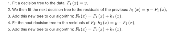
参考https://zhuanlan.zhihu.com/p/563409014

• Xgboost

• LightBGM