[足式机器人]Part4 南科大高等机器人控制课 Ch09 Dynamics of Open Chains
本文仅供学习使用
本文参考:
B站:CLEAR_LAB
笔者带更新-运动学
课程主讲教师:
Prof. Wei Zhang
南科大高等机器人控制课 Ch09 Dynamics of Open Chains
1. Introduction
1.1 From Single Rigid Body to Open Chains
- Recall Newton-Euler Equation for a single rigid body:
F = d d t H = I A + V ~ ? I V \mathcal{F} =\frac{\mathrm{d}}{\mathrm{d}t}\mathcal{H} =\mathcal{I} \mathcal{A} +\tilde{\mathcal{V}}^*\mathcal{I} \mathcal{V} F=dtd?H=IA+V~?IV - Open chains consists of multiple rigid links connected through joints
- Dynamics of adjacent links are coupled
- This lecture: model multi-body dynamics subject to joint constrainsts.
1.2 Preview of Open-Chain Dynamics
-
Equations of Motion are a set of 2nd-order differential equations:
τ = M ( θ ) θ ¨ + c ( θ , θ ˙ ) \tau =M\left( \theta \right) \ddot{\theta}+c\left( \theta ,\dot{\theta} \right) τ=M(θ)θ¨+c(θ,θ˙)
θ ∈ R n \theta \in \mathbb{R} ^n θ∈Rn : vector of joint variables ;
τ ∈ R n \tau \in \mathbb{R} ^n τ∈Rn : vector of joint forces/torques(与之前的符号不一致);
M ( θ ) ∈ R n × n M\left( \theta \right) \in \mathbb{R} ^{n\times n} M(θ)∈Rn×n : mass matrix
c ( θ , θ ˙ ) ∈ R n c\left( \theta ,\dot{\theta} \right) \in \mathbb{R} ^n c(θ,θ˙)∈Rn : forces that lump together centripetal, Coriolis, gravity, friction terms, and torques induced by external forces. These terms depends on θ \theta θ and θ ˙ \dot{\theta} θ˙ -
Forward dynamics : Determine accecleration θ ¨ \ddot{\theta} θ¨ given the state ( θ , θ ˙ ) \left( \theta ,\dot{\theta} \right) (θ,θ˙) and the joint forces/torques
θ ¨ ← F D ( τ , θ , θ ˙ , F e x t ) \ddot{\theta}\gets FD\left( \tau ,\theta ,\dot{\theta},\mathcal{F} _{\mathrm{ext}} \right) θ¨←FD(τ,θ,θ˙,Fext?) -
Inverse dynamics : Finding torques/forces given state ( θ , θ ˙ ) \left( \theta ,\dot{\theta} \right) (θ,θ˙) and desired acceleration θ ¨ \ddot{\theta} θ¨ (Given desired motion, find the required torque to generate the desired motion)
τ ← I D ( θ , θ ˙ , θ ¨ , F e x t ) \tau \gets ID\left( \theta ,\dot{\theta},\ddot{\theta},\mathcal{F} _{\mathrm{ext}} \right) τ←ID(θ,θ˙,θ¨,Fext?)
1.3 Lagrangian VS. Newton-Euler Methods
- There are typically two ways to derive the equation of motion for an open-chain robot: Lagrangian method and Newton-Euler method
Lagrangian Formulation : Energy-based method ; Dynamic equations in closed form ; Often used for study of dynamic properties and analysis of control methods
Newton-Euler Formulation : Balance of forces/torques ; Dynamic equations in numeric/recuisive form ; Often used for numerical solution of forward/inverse dynamics
We focus on Newton-Euler Formulation
2. Inverse Dynamics: Recursive Newton-Euler Algorithm(RNEA)
2.1 RNEA: Notations

-
Number bodies : 1 to N N N
Parents : p ( i ) : p ( 3 ) = { 2 } , p ( 4 ) = { 2 } p\left( i \right) :p\left( 3 \right) =\left\{ 2 \right\} ,p\left( 4 \right) =\left\{ 2 \right\} p(i):p(3)={2},p(4)={2}
Children : c ( i ) : c ( 2 ) = { 3 , 4 } , c ( 1 ) = { 2 } c\left( i \right) :c\left( 2 \right) =\left\{ 3,4 \right\} ,c\left( 1 \right) =\left\{ 2 \right\} c(i):c(2)={3,4},c(1)={2} -
Joint i i i connects p ( i ) p\left( i \right) p(i) to i i i
-
Frame { i } \left\{ i \right\} {i} attached to body i i i at the joint
-
S i \mathcal{S} _{\mathrm{i}} Si? : Spatial velocity (screw axis) of joint i i i
-
V i \mathcal{V} _{\mathrm{i}} Vi? and A i \mathcal{A} _{\mathrm{i}} Ai? : spatial velocity and acceleration of body i i i
-
F i \mathcal{F} _{\mathrm{i}} Fi? : force(wrench) onto body i i i from body p ( i ) p\left( i \right) p(i)
-
Note : By default, all vectors ( S i , V i , F i ) \left( \mathcal{S} _{\mathrm{i}},\mathcal{V} _{\mathrm{i}},\mathcal{F} _{\mathrm{i}} \right) (Si?,Vi?,Fi?) are expressed in local frame { i } \left\{ i \right\} {i}
2.1.1 RNEA: Velocity and Accel. Propagation(Forward Pass)
Goal: Given joint velocity θ ˙ \dot{\theta} θ˙ and acceleration θ ¨ \ddot{\theta} θ¨ , compute the body spatial velocity V i \mathcal{V} _{\mathrm{i}} Vi? and spatial acceleration A i \mathcal{A} _{\mathrm{i}} Ai?
- Velocity Propagation : V i i = [ X p ( i ) i ] V p ( i ) p ( i ) + S i i θ ˙ i \mathcal{V} _{\mathrm{i}}^{i}=\left[ X_{\mathrm{p}\left( i \right)}^{i} \right] \mathcal{V} _{\mathrm{p}\left( i \right)}^{p\left( i \right)}+\mathcal{S} _{\mathrm{i}}^{i}\dot{\theta}_{\mathrm{i}} Vii?=[Xp(i)i?]Vp(i)p(i)?+Sii?θ˙i?
- Accel Propagation : A i i = [ X p ( i ) i ] A p ( i ) p ( i ) + V ~ i i S i i θ ˙ i + S i i θ ¨ i \mathcal{A} _{\mathrm{i}}^{i}=\left[ X_{\mathrm{p}\left( i \right)}^{i} \right] \mathcal{A} _{\mathrm{p}\left( i \right)}^{p\left( i \right)}+\tilde{\mathcal{V}}_{\mathrm{i}}^{i}\mathcal{S} _{\mathrm{i}}^{i}\dot{\theta}_{\mathrm{i}}+\mathcal{S} _{\mathrm{i}}^{i}\ddot{\theta}_{\mathrm{i}} Aii?=[Xp(i)i?]Ap(i)p(i)?+V~ii?Sii?θ˙i?+Sii?θ¨i?
从机架侧开始计算
2.1.2 RNEA: Force Propagation(Backward Pass)
Goal : Given body spatial velocity V i \mathcal{V} _{\mathrm{i}} Vi? amd spatial acceleration A i \mathcal{A} _{\mathrm{i}} Ai?, compute the joint wrench F i \mathcal{F} _{\mathrm{i}} Fi? and the corresponding torque τ i = S i T F i \tau _{\mathrm{i}}={\mathcal{S} _{\mathrm{i}}}^{\mathrm{T}}\mathcal{F} _{\mathrm{i}} τi?=Si?TFi?
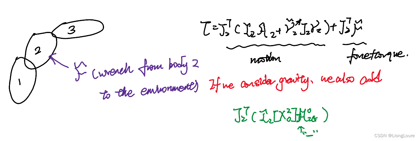
{ F i = I i A i + V ~ i ? I i V i + ∑ j ∈ c ( i ) F j τ i = S i T F i \begin{cases} \mathcal{F} _{\mathrm{i}}=\mathcal{I} _{\mathrm{i}}\mathcal{A} _{\mathrm{i}}+{\tilde{\mathcal{V}}_{\mathrm{i}}}^*\mathcal{I} _{\mathrm{i}}\mathcal{V} _{\mathrm{i}}+\sum\nolimits_{j\in c\left( i \right)}^{}{\mathcal{F} _{\mathrm{j}}}\\ \tau _{\mathrm{i}}={\mathcal{S} _{\mathrm{i}}}^{\mathrm{T}}\mathcal{F} _{\mathrm{i}}\\ \end{cases} {Fi?=Ii?Ai?+V~i??Ii?Vi?+∑j∈c(i)?Fj?τi?=Si?TFi??
从末端执行构件处开始计算:
- Body 4:
F 4 + F G 4 = I 4 A 4 + V ~ 4 ? I 4 V 4 ? F 4 = I 4 A 4 + V ~ 4 ? I 4 V 4 ? F G 4 , F G 4 = I 4 A G 4 = I 4 [ X O 4 ] A G O \mathcal{F} _4+\mathcal{F} _{\mathrm{G}4}=\mathcal{I} _4\mathcal{A} _4+{\tilde{\mathcal{V}}_4}^*\mathcal{I} _4\mathcal{V} _4 \\ \Rightarrow \mathcal{F} _4=\mathcal{I} _4\mathcal{A} _4+{\tilde{\mathcal{V}}_4}^*\mathcal{I} _4\mathcal{V} _4-\mathcal{F} _{\mathrm{G}4},\mathcal{F} _{\mathrm{G}4}=\mathcal{I} _4\mathcal{A} _{\mathrm{G}}^{4}=\mathcal{I} _4\left[ X_{\mathrm{O}}^{4} \right] \mathcal{A} _{\mathrm{G}}^{O} F4?+FG4?=I4?A4?+V~4??I4?V4??F4?=I4?A4?+V~4??I4?V4??FG4?,FG4?=I4?AG4?=I4?[XO4?]AGO?
τ 4 = S 4 T F 4 \tau _4={\mathcal{S} _4}^{\mathrm{T}}\mathcal{F} _4 τ4?=S4?TF4? - Body 2:
F 2 = I 2 A 2 + V ~ 2 ? I 2 V 2 + F 4 + F 3 ? F G 2 , F G 2 = I 2 [ X O 2 ] A G 2 O τ 2 = S 2 T F 2 \mathcal{F} _2=\mathcal{I} _2\mathcal{A} _2+{\tilde{\mathcal{V}}_2}^*\mathcal{I} _2\mathcal{V} _2+\mathcal{F} _4+\mathcal{F} _3-\mathcal{F} _{\mathrm{G}2},\mathcal{F} _{\mathrm{G}2}=\mathcal{I} _2\left[ X_{\mathrm{O}}^{2} \right] \mathcal{A} _{\mathrm{G}2}^{O} \\ \tau _2={\mathcal{S} _2}^{\mathrm{T}}\mathcal{F} _2 F2?=I2?A2?+V~2??I2?V2?+F4?+F3??FG2?,FG2?=I2?[XO2?]AG2O?τ2?=S2?TF2?
2.1.3 Recursive Newton-Euler Algorithm
τ
←
R
N
E
A
(
θ
,
θ
˙
,
θ
¨
,
F
e
x
t
;
M
o
d
e
l
)
\tau \gets RNEA\left( \theta ,\dot{\theta},\ddot{\theta},\mathcal{F} _{\mathrm{ext}};Model \right)
τ←RNEA(θ,θ˙,θ¨,Fext?;Model)
Initialize :
V
0
=
0
,
A
0
=
?
A
G
\mathcal{V} _0=0,\mathcal{A} _0=-\mathcal{A} _{\mathrm{G}}
V0?=0,A0?=?AG? (without gravity “trick” modify
F
i
=
I
i
A
i
+
V
~
i
?
I
i
V
i
?
I
i
[
X
O
i
]
A
G
i
O
\mathcal{F} _{\mathrm{i}}=\mathcal{I} _{\mathrm{i}}\mathcal{A} _{\mathrm{i}}+{\tilde{\mathcal{V}}_{\mathrm{i}}}^*\mathcal{I} _{\mathrm{i}}\mathcal{V} _{\mathrm{i}}-\mathcal{I} _{\mathrm{i}}\left[ X_{\mathrm{O}}^{i} \right] \mathcal{A} _{\mathrm{Gi}}^{O}
Fi?=Ii?Ai?+V~i??Ii?Vi??Ii?[XOi?]AGiO?)
- Forward pass : For
i
=
1
i=1
i=1 to
N
N
N
V i i = [ X p ( i ) i ] V p ( i ) p ( i ) + S i i θ ˙ i \mathcal{V} _{\mathrm{i}}^{i}=\left[ X_{\mathrm{p}\left( i \right)}^{i} \right] \mathcal{V} _{\mathrm{p}\left( i \right)}^{p\left( i \right)}+\mathcal{S} _{\mathrm{i}}^{i}\dot{\theta}_{\mathrm{i}} Vii?=[Xp(i)i?]Vp(i)p(i)?+Sii?θ˙i?
A i i = [ X p ( i ) i ] A p ( i ) p ( i ) + V ~ i i S i i θ ˙ i + S i i θ ¨ i \mathcal{A} _{\mathrm{i}}^{i}=\left[ X_{\mathrm{p}\left( i \right)}^{i} \right] \mathcal{A} _{\mathrm{p}\left( i \right)}^{p\left( i \right)}+\tilde{\mathcal{V}}_{\mathrm{i}}^{i}\mathcal{S} _{\mathrm{i}}^{i}\dot{\theta}_{\mathrm{i}}+\mathcal{S} _{\mathrm{i}}^{i}\ddot{\theta}_{\mathrm{i}} Aii?=[Xp(i)i?]Ap(i)p(i)?+V~ii?Sii?θ˙i?+Sii?θ¨i?
F i = I i A i + V ~ i ? I i V i \mathcal{F} _{\mathrm{i}}=\mathcal{I} _{\mathrm{i}}\mathcal{A} _{\mathrm{i}}+{\tilde{\mathcal{V}}_{\mathrm{i}}}^*\mathcal{I} _{\mathrm{i}}\mathcal{V} _{\mathrm{i}} Fi?=Ii?Ai?+V~i??Ii?Vi? - Backward pass : For
i
=
N
i=N
i=N to 1
τ i = S i T F i \tau _{\mathrm{i}}={\mathcal{S} _{\mathrm{i}}}^{\mathrm{T}}\mathcal{F} _{\mathrm{i}} τi?=Si?TFi?
F p ( i ) = F p ( i ) + [ X i p ( i ) ] F i \mathcal{F} _{\mathrm{p}\left( i \right)}=\mathcal{F} _{\mathrm{p}\left( i \right)}+\left[ X_{\mathrm{i}}^{p\left( i \right)} \right] \mathcal{F} _{\mathrm{i}} Fp(i)?=Fp(i)?+[Xip(i)?]Fi?
3. Analytical Form of the Dynamics Model
3.1 Structures in Dynamic Equation
Jacobian of each link(body) :
J
1
,
?
?
,
J
4
J_1,\cdots ,J_4
J1?,?,J4?
J
i
J_{\mathrm{i}}
Ji? : denote the Jacobian of body(Link)
i
i
i , i.e.
V
i
=
J
i
θ
˙
=
[
J
i
1
J
i
2
J
i
3
J
i
4
]
[
θ
˙
1
θ
˙
2
θ
˙
3
θ
˙
4
]
\mathcal{V} _{\mathrm{i}}=J_{\mathrm{i}}\dot{\theta}=\left[ \begin{matrix} J_{\mathrm{i}1}& J_{\mathrm{i}2}& J_{\mathrm{i}3}& J_{\mathrm{i}4}\\ \end{matrix} \right] \left[ \begin{array}{c} \dot{\theta}_1\\ \dot{\theta}_2\\ \dot{\theta}_3\\ \dot{\theta}_4\\ \end{array} \right]
Vi?=Ji?θ˙=[Ji1??Ji2??Ji3??Ji4??]
?θ˙1?θ˙2?θ˙3?θ˙4??
?
e.g.
V
1
=
J
1
θ
˙
=
[
δ
11
S
1
δ
12
S
2
δ
13
S
3
δ
14
S
4
]
[
θ
˙
1
θ
˙
2
θ
˙
3
θ
˙
4
]
=
[
S
1
0
0
0
]
[
θ
˙
1
θ
˙
2
θ
˙
3
θ
˙
4
]
δ
i
j
=
{
1
,
i
f
??
j
o
i
n
t
??
j
s
u
p
p
o
r
t
??
b
o
d
y
??
i
0
,
o
t
h
e
r
w
i
s
e
\mathcal{V} _1=J_1\dot{\theta}=\left[ \begin{matrix} \delta _{11}\mathcal{S} _1& \delta _{12}\mathcal{S} _2& \delta _{13}\mathcal{S} _3& \delta _{14}\mathcal{S} _4\\ \end{matrix} \right] \left[ \begin{array}{c} \dot{\theta}_1\\ \dot{\theta}_2\\ \dot{\theta}_3\\ \dot{\theta}_4\\ \end{array} \right] =\left[ \begin{matrix} \mathcal{S} _1& 0& 0& 0\\ \end{matrix} \right] \left[ \begin{array}{c} \dot{\theta}_1\\ \dot{\theta}_2\\ \dot{\theta}_3\\ \dot{\theta}_4\\ \end{array} \right] \\ \delta _{\mathrm{ij}}=\begin{cases} 1, if\,\,joint\,\,\mathrm{j} support\,\,body\,\,\mathrm{i}\\ 0, otherwise\\ \end{cases}
V1?=J1?θ˙=[δ11?S1??δ12?S2??δ13?S3??δ14?S4??]
?θ˙1?θ˙2?θ˙3?θ˙4??
?=[S1??0?0?0?]
?θ˙1?θ˙2?θ˙3?θ˙4??
?δij?={1,ifjointjsupportbodyi0,otherwise?
V 2 = J 2 θ ˙ = [ S 1 S 2 0 0 ] θ ˙ ? V 2 2 = [ [ X 1 2 ] S 2 1 S 2 2 0 0 ] θ ˙ \mathcal{V} _2=J_2\dot{\theta}=\left[ \begin{matrix} \mathcal{S} _1& \mathcal{S} _2& 0& 0\\ \end{matrix} \right] \dot{\theta}\Rightarrow \mathcal{V} _{2}^{2}=\left[ \left[ X_{1}^{2} \right] \begin{matrix} \mathcal{S} _{2}^{1}& \mathcal{S} _{2}^{2}& 0& 0\\ \end{matrix} \right] \dot{\theta} V2?=J2?θ˙=[S1??S2??0?0?]θ˙?V22?=[[X12?]S21??S22??0?0?]θ˙
see the two-body example:
- Forward pass :
V 1 = S 1 θ ˙ 1 \mathcal{V} _1=\mathcal{S} _1\dot{\theta}_1 V1?=S1?θ˙1? , V 2 2 = [ [ X 1 2 ] S 2 1 S 2 2 ] [ θ ˙ 1 θ ˙ 2 ] \mathcal{V} _{2}^{2}=\left[ \begin{matrix} \left[ X_{1}^{2} \right] \mathcal{S} _{2}^{1}& \mathcal{S} _{2}^{2}\\ \end{matrix} \right] \left[ \begin{array}{c} \dot{\theta}_1\\ \dot{\theta}_2\\ \end{array} \right] V22?=[[X12?]S21??S22??][θ˙1?θ˙2??]
A 1 , A 2 \mathcal{A} _1, \mathcal{A} _2 A1?,A2? - Backward pass :
F 2 = I 2 A 2 + V ~ 2 ? I 2 V 2 ? F 2 e x t ? F 2 G F 1 = I 1 A 1 + V ~ 1 ? I 1 V 1 ? F 1 e x t ? F 1 G + [ X 2 1 ] ( I 2 A 2 + V ~ 2 ? I 2 V 2 ? F 2 e x t ? F 2 G ) τ 2 = S 2 T F 2 τ 1 = S 1 T F 1 \mathcal{F} _2=\mathcal{I} _2\mathcal{A} _2+{\tilde{\mathcal{V}}_2}^*\mathcal{I} _2\mathcal{V} _2-\mathcal{F} _{2\mathrm{ext}}-\mathcal{F} _{2\mathrm{G}} \\ \mathcal{F} _1=\mathcal{I} _1\mathcal{A} _1+{\tilde{\mathcal{V}}_1}^*\mathcal{I} _1\mathcal{V} _1-\mathcal{F} _{1\mathrm{ext}}-\mathcal{F} _{1\mathrm{G}}+\left[ X_{2}^{1} \right] \left( \mathcal{I} _2\mathcal{A} _2+{\tilde{\mathcal{V}}_2}^*\mathcal{I} _2\mathcal{V} _2-\mathcal{F} _{2\mathrm{ext}}-\mathcal{F} _{2\mathrm{G}} \right) \\ \tau _2={\mathcal{S} _2}^{\mathrm{T}}\mathcal{F} _2 \\ \tau _1={\mathcal{S} _1}^{\mathrm{T}}\mathcal{F} _1 F2?=I2?A2?+V~2??I2?V2??F2ext??F2G?F1?=I1?A1?+V~1??I1?V1??F1ext??F1G?+[X21?](I2?A2?+V~2??I2?V2??F2ext??F2G?)τ2?=S2?TF2?τ1?=S1?TF1?
Overall torque expression :
τ
1
=
S
1
T
F
1
=
S
1
T
(
I
1
A
1
+
V
~
1
?
I
1
V
1
?
F
1
e
x
t
?
F
1
G
+
[
X
2
1
]
(
I
2
A
2
+
V
~
2
?
I
2
V
2
?
F
2
e
x
t
?
F
2
G
)
)
=
S
1
T
(
I
1
A
1
+
V
~
1
?
I
1
V
1
)
+
(
[
X
1
2
]
S
1
)
T
(
I
2
A
2
+
V
~
2
?
I
2
V
2
)
?
S
1
T
(
F
1
e
x
t
+
F
1
G
+
[
X
2
1
]
(
F
2
e
x
t
+
F
2
G
)
)
\tau _1={\mathcal{S} _1}^{\mathrm{T}}\mathcal{F} _1={\mathcal{S} _1}^{\mathrm{T}}\left( \mathcal{I} _1\mathcal{A} _1+{\tilde{\mathcal{V}}_1}^*\mathcal{I} _1\mathcal{V} _1-\mathcal{F} _{1\mathrm{ext}}-\mathcal{F} _{1\mathrm{G}}+\left[ X_{2}^{1} \right] \left( \mathcal{I} _2\mathcal{A} _2+{\tilde{\mathcal{V}}_2}^*\mathcal{I} _2\mathcal{V} _2-\mathcal{F} _{2\mathrm{ext}}-\mathcal{F} _{2\mathrm{G}} \right) \right) \\ ={\mathcal{S} _1}^{\mathrm{T}}\left( \mathcal{I} _1\mathcal{A} _1+{\tilde{\mathcal{V}}_1}^*\mathcal{I} _1\mathcal{V} _1 \right) +\left( \left[ X_{1}^{2} \right] \mathcal{S} _1 \right) ^{\mathrm{T}}\left( \mathcal{I} _2\mathcal{A} _2+{\tilde{\mathcal{V}}_2}^*\mathcal{I} _2\mathcal{V} _2 \right) -{\mathcal{S} _1}^{\mathrm{T}}\left( \mathcal{F} _{1\mathrm{ext}}+\mathcal{F} _{1\mathrm{G}}+\left[ X_{2}^{1} \right] \left( \mathcal{F} _{2\mathrm{ext}}+\mathcal{F} _{2\mathrm{G}} \right) \right)
τ1?=S1?TF1?=S1?T(I1?A1?+V~1??I1?V1??F1ext??F1G?+[X21?](I2?A2?+V~2??I2?V2??F2ext??F2G?))=S1?T(I1?A1?+V~1??I1?V1?)+([X12?]S1?)T(I2?A2?+V~2??I2?V2?)?S1?T(F1ext?+F1G?+[X21?](F2ext?+F2G?))
due to motion of body 1 and 2 and external force of body 1 and 2
τ = [ τ 1 τ 2 ] = [ S 1 T ( I 1 A 1 + V ~ 1 ? I 1 V 1 ) + ( [ X 1 2 ] S 1 ) T ( I 2 A 2 + V ~ 2 ? I 2 V 2 ) ? S 1 T ( F 1 e x t + F 1 G + [ X 2 1 ] ( F 2 e x t + F 2 G ) ) S 2 T ( I 2 A 2 + V ~ 2 ? I 2 V 2 ? F 2 e x t ? F 2 G ) ] = [ S 1 T 0 ] ( I 1 A 1 + V ~ 1 ? I 1 V 1 ? F 1 e x t ? F 1 G ) + [ ( [ X 1 2 ] S 1 ) T S 2 T ] ( I 2 A 2 + V ~ 2 ? I 2 V 2 ? F 2 e x t ? F 2 G ) = J 1 T ( I 1 A 1 + V ~ 1 ? I 1 V 1 ? F 1 e x t ? F 1 G ) + J 2 T ( I 2 A 2 + V ~ 2 ? I 2 V 2 ? F 2 e x t ? F 2 G ) \tau =\left[ \begin{array}{c} \tau _1\\ \tau _2\\ \end{array} \right] =\left[ \begin{array}{c} {\mathcal{S} _1}^{\mathrm{T}}\left( \mathcal{I} _1\mathcal{A} _1+{\tilde{\mathcal{V}}_1}^*\mathcal{I} _1\mathcal{V} _1 \right) +\left( \left[ X_{1}^{2} \right] \mathcal{S} _1 \right) ^{\mathrm{T}}\left( \mathcal{I} _2\mathcal{A} _2+{\tilde{\mathcal{V}}_2}^*\mathcal{I} _2\mathcal{V} _2 \right) -{\mathcal{S} _1}^{\mathrm{T}}\left( \mathcal{F} _{1\mathrm{ext}}+\mathcal{F} _{1\mathrm{G}}+\left[ X_{2}^{1} \right] \left( \mathcal{F} _{2\mathrm{ext}}+\mathcal{F} _{2\mathrm{G}} \right) \right)\\ {\mathcal{S} _2}^{\mathrm{T}}\left( \mathcal{I} _2\mathcal{A} _2+{\tilde{\mathcal{V}}_2}^*\mathcal{I} _2\mathcal{V} _2-\mathcal{F} _{2\mathrm{ext}}-\mathcal{F} _{2\mathrm{G}} \right)\\ \end{array} \right] \\ =\left[ \begin{array}{c} {\mathcal{S} _1}^{\mathrm{T}}\\ 0\\ \end{array} \right] \left( \mathcal{I} _1\mathcal{A} _1+{\tilde{\mathcal{V}}_1}^*\mathcal{I} _1\mathcal{V} _1-\mathcal{F} _{1\mathrm{ext}}-\mathcal{F} _{1\mathrm{G}} \right) +\left[ \begin{array}{c} \left( \left[ X_{1}^{2} \right] \mathcal{S} _1 \right) ^{\mathrm{T}}\\ {\mathcal{S} _2}^{\mathrm{T}}\\ \end{array} \right] \left( \mathcal{I} _2\mathcal{A} _2+{\tilde{\mathcal{V}}_2}^*\mathcal{I} _2\mathcal{V} _2-\mathcal{F} _{2\mathrm{ext}}-\mathcal{F} _{2\mathrm{G}} \right) \\ ={J_1}^{\mathrm{T}}\left( \mathcal{I} _1\mathcal{A} _1+{\tilde{\mathcal{V}}_1}^*\mathcal{I} _1\mathcal{V} _1-\mathcal{F} _{1\mathrm{ext}}-\mathcal{F} _{1\mathrm{G}} \right) +{J_2}^{\mathrm{T}}\left( \mathcal{I} _2\mathcal{A} _2+{\tilde{\mathcal{V}}_2}^*\mathcal{I} _2\mathcal{V} _2-\mathcal{F} _{2\mathrm{ext}}-\mathcal{F} _{2\mathrm{G}} \right) τ=[τ1?τ2??]= ?S1?T(I1?A1?+V~1??I1?V1?)+([X12?]S1?)T(I2?A2?+V~2??I2?V2?)?S1?T(F1ext?+F1G?+[X21?](F2ext?+F2G?))S2?T(I2?A2?+V~2??I2?V2??F2ext??F2G?)? ?=[S1?T0?](I1?A1?+V~1??I1?V1??F1ext??F1G?)+[([X12?]S1?)TS2?T?](I2?A2?+V~2??I2?V2??F2ext??F2G?)=J1?T(I1?A1?+V~1??I1?V1??F1ext??F1G?)+J2?T(I2?A2?+V~2??I2?V2??F2ext??F2G?)
Overall : in general with N-links / Joints
τ = ∑ i = 1 N J i T ( I i A i + V ~ i ? I i V i ? F i e x t ? F i G ) \tau =\sum_{i=1}^N{{J_{\mathrm{i}}}^{\mathrm{T}}\left( \mathcal{I} _{\mathrm{i}}\mathcal{A} _{\mathrm{i}}+{\tilde{\mathcal{V}}_{\mathrm{i}}}^*\mathcal{I} _{\mathrm{i}}\mathcal{V} _{\mathrm{i}}-\mathcal{F} _{\mathrm{iext}}-\mathcal{F} _{\mathrm{iG}} \right)} τ=i=1∑N?Ji?T(Ii?Ai?+V~i??Ii?Vi??Fiext??FiG?)
V i = J i θ ˙ A i = V ˙ i = ( J ˙ i θ ˙ + J i θ ¨ + V ~ i J i θ ˙ ) \mathcal{V} _{\mathrm{i}}=J_{\mathrm{i}}\dot{\theta} \\ \mathcal{A} _{\mathrm{i}}=\dot{\mathcal{V}}_{\mathrm{i}}=\left( \dot{J}_{\mathrm{i}}\dot{\theta}+J_{\mathrm{i}}\ddot{\theta}+\tilde{\mathcal{V}}_{\mathrm{i}}J_{\mathrm{i}}\dot{\theta} \right) Vi?=Ji?θ˙Ai?=V˙i?=(J˙i?θ˙+Ji?θ¨+V~i?Ji?θ˙)
上式看上去难以理解,尤其是加速度旋量,本质上是因为在构件坐标系下的求导,相当于需要对运动基向量求导所产生的加速度
带入可得:
τ
=
∑
i
=
1
N
J
i
T
I
i
J
i
θ
¨
+
∑
i
=
1
N
J
i
T
(
I
i
J
˙
i
+
I
i
V
~
i
J
i
+
V
~
i
?
I
i
J
i
)
θ
˙
\tau =\sum_{i=1}^N{{J_{\mathrm{i}}}^{\mathrm{T}}\mathcal{I} _{\mathrm{i}}J_{\mathrm{i}}}\ddot{\theta}+\sum_{i=1}^N{{J_{\mathrm{i}}}^{\mathrm{T}}\left( \mathcal{I} _{\mathrm{i}}\dot{J}_{\mathrm{i}}+\mathcal{I} _{\mathrm{i}}\tilde{\mathcal{V}}_{\mathrm{i}}J_{\mathrm{i}}+{\tilde{\mathcal{V}}_{\mathrm{i}}}^*\mathcal{I} _{\mathrm{i}}J_{\mathrm{i}} \right)}\dot{\theta}
τ=i=1∑N?Ji?TIi?Ji?θ¨+i=1∑N?Ji?T(Ii?J˙i?+Ii?V~i?Ji?+V~i??Ii?Ji?)θ˙
∑
i
=
1
N
J
i
T
I
i
J
i
=
M
(
θ
)
,
∑
i
=
1
N
J
i
T
(
I
i
J
˙
i
+
I
i
V
~
i
J
i
+
V
~
i
?
I
i
J
i
)
=
c
(
θ
,
θ
˙
)
\sum_{i=1}^N{{J_{\mathrm{i}}}^{\mathrm{T}}\mathcal{I} _{\mathrm{i}}J_{\mathrm{i}}}=M\left( \theta \right) ,\sum_{i=1}^N{{J_{\mathrm{i}}}^{\mathrm{T}}\left( \mathcal{I} _{\mathrm{i}}\dot{J}_{\mathrm{i}}+\mathcal{I} _{\mathrm{i}}\tilde{\mathcal{V}}_{\mathrm{i}}J_{\mathrm{i}}+{\tilde{\mathcal{V}}_{\mathrm{i}}}^*\mathcal{I} _{\mathrm{i}}J_{\mathrm{i}} \right)}=c\left( \theta ,\dot{\theta} \right)
∑i=1N?Ji?TIi?Ji?=M(θ),∑i=1N?Ji?T(Ii?J˙i?+Ii?V~i?Ji?+V~i??Ii?Ji?)=c(θ,θ˙) ,
τ
G
=
∑
i
=
1
N
J
i
T
I
i
[
X
O
i
]
(
?
A
i
G
O
)
\tau _G=\sum_{i=1}^N{{J_{\mathrm{i}}}^{\mathrm{T}}\mathcal{I} _{\mathrm{i}}\left[ X_{\mathrm{O}}^{i} \right]}\left( -\mathcal{A} _{\mathrm{iG}}^{O} \right)
τG?=∑i=1N?Ji?TIi?[XOi?](?AiGO?)
最终理解:
τ
=
M
(
θ
)
θ
¨
+
c
(
θ
,
θ
˙
)
θ
˙
+
τ
G
+
J
T
(
θ
)
F
e
x
t
\tau =M\left( \theta \right) \ddot{\theta}+c\left( \theta ,\dot{\theta} \right) \dot{\theta}+\tau _G+J^{\mathrm{T}}\left( \theta \right) \mathcal{F} _{\mathrm{ext}}
τ=M(θ)θ¨+c(θ,θ˙)θ˙+τG?+JT(θ)Fext?
F
e
x
t
\mathcal{F} _{\mathrm{ext}}
Fext? : applied from the body to environment
回顾:
J i J_{\mathrm{i}} Ji? : body/link i Jacobian , V i ∣ 6 × 1 = J i ∣ 6 × n θ ˙ ∣ n × 1 \left. \mathcal{V} _{\mathrm{i}} \right|_{6\times 1}=\left. J_{\mathrm{i}} \right|_{6\times \mathrm{n}}\left. \dot{\theta} \right|_{\mathrm{n}\times 1} Vi?∣6×1?=Ji?∣6×n?θ˙ ?n×1?
τ ∈ R n \tau \in \mathbb{R} ^n τ∈Rn , τ \tau τ play two major roles :
- generate motion
- generate force/torque
3.2 Properties of Dynamics Model of Multi-Body Systems
Only cpnsider body 2’s effect
4. Forward Dynamics Algorithms
4.1 Forward Dynamics Problem
τ = M ( θ ) θ ¨ + c ( θ , θ ˙ ) θ ˙ + τ G + J T ( θ ) F e x t = M ( θ ) θ ¨ + h ( θ , θ ˙ ) \tau =M\left( \theta \right) \ddot{\theta}+c\left( \theta ,\dot{\theta} \right) \dot{\theta}+\tau _G+J^{\mathrm{T}}\left( \theta \right) \mathcal{F} _{\mathrm{ext}}=M\left( \theta \right) \ddot{\theta}+h\left( \theta ,\dot{\theta} \right) τ=M(θ)θ¨+c(θ,θ˙)θ˙+τG?+JT(θ)Fext?=M(θ)θ¨+h(θ,θ˙)
-
Inverse dynamics : τ ← R N E A ( θ , θ ˙ , θ ¨ , F e x t ) \tau \gets RNEA\left( \theta ,\dot{\theta},\ddot{\theta},\mathcal{F} _{\mathrm{ext}} \right) τ←RNEA(θ,θ˙,θ¨,Fext?) —— O ( N ) O\left( N \right) O(N) complexity
RNEA can work directly with a givenURDF-United Robotics Description Formatmodel (kinematic tree + joint model + dynamic parameters). It does not require explicit formula for M ( θ ) , h ( θ , θ ˙ ) M\left( \theta \right),h\left( \theta ,\dot{\theta} \right) M(θ),h(θ,θ˙) -
Forward dynamics : Given ( θ , θ ˙ ) , τ , F e x t \left( \theta ,\dot{\theta} \right) ,\tau ,\mathcal{F} _{\mathrm{ext}} (θ,θ˙),τ,Fext? , find θ ¨ \ddot{\theta} θ¨
Calculate h ( θ , θ ˙ ) = c ( θ , θ ˙ ) θ ˙ + τ G + J T F e x t h\left( \theta ,\dot{\theta} \right) =c\left( \theta ,\dot{\theta} \right) \dot{\theta}+\tau _{\mathrm{G}}+J^{\mathrm{T}}\mathcal{F} _{\mathrm{ext}} h(θ,θ˙)=c(θ,θ˙)θ˙+τG?+JTFext?
Caculate mass matrix M ( θ ) = ∑ i = 1 N J i T I i J i M\left( \theta \right) =\sum_{i=1}^N{{J_{\mathrm{i}}}^{\mathrm{T}}\mathcal{I} _{\mathrm{i}}J_{\mathrm{i}}} M(θ)=∑i=1N?Ji?TIi?Ji?
Solve M θ ¨ = τ ? h ? θ ¨ = M ? 1 ( τ ? h ) M\ddot{\theta}=\tau -h\Rightarrow \ddot{\theta}=M^{-1}\left( \tau -h \right) Mθ¨=τ?h?θ¨=M?1(τ?h): This is not the most efficient way to find θ ¨ \ddot{\theta} θ¨
4.2 Caculations of h and M
Denote our inverse dynamics algorithm : τ = R N E A ( θ , θ ˙ , θ ¨ , F e x t ) = M θ ¨ + h \tau =RNEA\left( \theta ,\dot{\theta},\ddot{\theta},\mathcal{F} _{\mathrm{ext}} \right) =M\ddot{\theta}+h τ=RNEA(θ,θ˙,θ¨,Fext?)=Mθ¨+h
-
Calculation of h h h : obviously , τ = h \tau =h τ=h if θ ¨ = 0 \ddot{\theta}=0 θ¨=0. Therefore, h h h can be computed via : h ( θ , θ ˙ ) = R N E A ( θ , θ ˙ , 0 , F e x t ) h\left( \theta ,\dot{\theta} \right) =RNEA\left( \theta ,\dot{\theta},0,\mathcal{F} _{\mathrm{ext}} \right) h(θ,θ˙)=RNEA(θ,θ˙,0,Fext?)
-
Calculation of M M M : Note h ( θ , θ ˙ ) = c ( θ , θ ˙ ) θ ˙ + τ G + J T F e x t h\left( \theta ,\dot{\theta} \right) =c\left( \theta ,\dot{\theta} \right) \dot{\theta}+\tau _{\mathrm{G}}+J^{\mathrm{T}}\mathcal{F} _{\mathrm{ext}} h(θ,θ˙)=c(θ,θ˙)θ˙+τG?+JTFext?
Set G = 0 , F e x t = 0 , θ ˙ = 0 G=0,\mathcal{F} _{\mathrm{ext}}=0,\dot{\theta}=0 G=0,Fext?=0,θ˙=0 , then h ( θ , θ ˙ ) = 0 h\left( \theta ,\dot{\theta} \right) =0 h(θ,θ˙)=0 , ? τ = M ( θ ) θ ¨ \Rightarrow \tau =M\left( \theta \right) \ddot{\theta} ?τ=M(θ)θ¨
We can compute the j j jth colum of M ( θ ) M\left( \theta \right) M(θ) by calling the inverse algorithm
τ = M : , j ( θ ) = R N E A ( 0 , 0 , θ ¨ 0 , j , 0 ) \tau =M_{:,\mathrm{j}}\left( \theta \right) =RNEA\left( 0,0,\ddot{\theta}_{0,\mathrm{j}},0 \right) τ=M:,j?(θ)=RNEA(0,0,θ¨0,j?,0) , θ ¨ 0 , j \ddot{\theta}_{0,\mathrm{j}} θ¨0,j? is a vector with all zeros except for a 1 at the j j jth entry
θ ¨ 0 , 1 = [ 1 0 ? 0 ] , τ = [ M 1 ( θ ) ? M n ( θ ) ] , M 1 , j ( θ ) = τ θ ¨ 0 , 1 \ddot{\theta}_{0,1}=\left[ \begin{array}{c} 1\\ 0\\ \vdots\\ 0\\ \end{array} \right] ,\tau =\left[ \begin{matrix} M_1\left( \theta \right)& \cdots& M_{\mathrm{n}}\left( \theta \right)\\ \end{matrix} \right] ,M_{1,\mathrm{j}}\left( \theta \right) =\tau \ddot{\theta}_{0,1} θ¨0,1?= ?10?0? ?,τ=[M1?(θ)???Mn?(θ)?],M1,j?(θ)=τθ¨0,1? -
A more effiicient algorithm for computing M M M is the
Composite-Rigid-Body Algorithm(CRBA). Details can be found in Featherstone’s Book
4.3 Forward Dynamics Algorithms
Now assume we have θ , θ ˙ , τ , M ( θ ) , h \theta ,\dot{\theta},\tau ,M\left( \theta \right) ,h θ,θ˙,τ,M(θ),h , then we can immediately compute θ ¨ \ddot{\theta} θ¨ as θ ¨ = M ? 1 ( τ ? h ) \ddot{\theta}=M^{-1}\left( \tau -h \right) θ¨=M?1(τ?h) —— θ ¨ = F D ( τ , θ , θ ˙ , F e x t ) \ddot{\theta}=FD\left( \tau ,\theta ,\dot{\theta},\mathcal{F} _{\mathrm{ext}} \right) θ¨=FD(τ,θ,θ˙,Fext?)
两种看似不同的求解思路,之间的关系是等同的
This provides a 2nd-order differential equation in R n \mathbb{R} ^n Rn , we can easily simulate the joint trajectory over any time period (under given ICs θ 0 , θ ˙ 0 \theta ^0,\dot{\theta}^0 θ0,θ˙0)
Computational Complexity:
RNEA :
O
(
N
)
O\left( N \right)
O(N)
h
(
θ
,
θ
˙
)
=
R
N
E
A
(
θ
,
θ
˙
,
0
,
F
e
x
t
)
h\left( \theta ,\dot{\theta} \right) =RNEA\left( \theta ,\dot{\theta},0,\mathcal{F} _{\mathrm{ext}} \right)
h(θ,θ˙)=RNEA(θ,θ˙,0,Fext?) :
O
(
N
)
O\left( N \right)
O(N)
M
(
θ
)
M\left( \theta \right)
M(θ) :
O
(
N
2
)
O\left( N^2 \right)
O(N2)
M
?
1
(
θ
)
M^{-1}\left( \theta \right)
M?1(θ) :
O
(
N
3
)
O\left( N^3 \right)
O(N3)
Most efficient forward dynamics algorithm :
Articulate-Body Algorithm(ABA): O ( N ) O\left( N \right) O(N)
4.4 More Discussions
M
(
θ
)
M\left( \theta \right)
M(θ) : Mass matrix ,
M
T
(
θ
)
=
M
(
θ
)
M^{\mathrm{T}}\left( \theta \right) =M\left( \theta \right)
MT(θ)=M(θ), also positive semi-definite.
M
(
θ
)
=
∑
i
=
1
N
J
i
T
I
i
J
i
M\left( \theta \right) =\sum_{i=1}^N{{J_{\mathrm{i}}}^{\mathrm{T}}\mathcal{I} _{\mathrm{i}}J_{\mathrm{i}}}
M(θ)=∑i=1N?Ji?TIi?Ji?——
I
i
\mathcal{I} _{\mathrm{i}}
Ii? Inertia matrix symmetric / postive semi-definite
There are many equivalent ways to define
c
(
θ
,
θ
˙
)
c\left( \theta ,\dot{\theta} \right)
c(θ,θ˙) , they are all related to the same product
c
(
θ
,
θ
˙
)
θ
˙
c\left( \theta ,\dot{\theta} \right) \dot{\theta}
c(θ,θ˙)θ˙ —— common and confusing
Typical expression for
c
c
c :
c
i
j
=
∑
k
=
1
1
2
(
?
M
i
j
?
θ
k
+
?
M
i
k
?
θ
j
?
?
M
j
k
?
θ
i
)
θ
˙
k
,
Γ
i
j
k
=
1
2
(
?
M
i
j
?
θ
k
+
?
M
i
k
?
θ
j
?
?
M
j
k
?
θ
i
)
c_{\mathrm{ij}}=\sum_{k=1}^{}{\frac{1}{2}\left( \frac{\partial M_{\mathrm{ij}}}{\partial \theta _{\mathrm{k}}}+\frac{\partial M_{\mathrm{ik}}}{\partial \theta _{\mathrm{j}}}-\frac{\partial M_{\mathrm{jk}}}{\partial \theta _{\mathrm{i}}} \right)}\dot{\theta}_{\mathrm{k}},\varGamma _{\mathrm{ijk}}=\frac{1}{2}\left( \frac{\partial M_{\mathrm{ij}}}{\partial \theta _{\mathrm{k}}}+\frac{\partial M_{\mathrm{ik}}}{\partial \theta _{\mathrm{j}}}-\frac{\partial M_{\mathrm{jk}}}{\partial \theta _{\mathrm{i}}} \right)
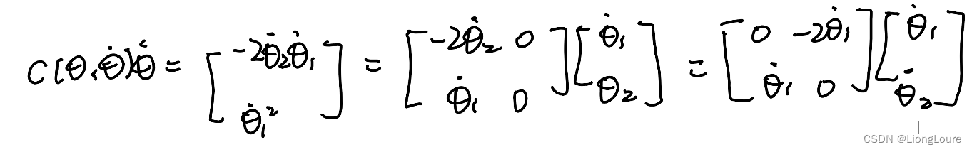
cij?=∑k=1?21?(?θk??Mij??+?θj??Mik????θi??Mjk??)θ˙k?,Γijk?=21?(?θk??Mij??+?θj??Mik????θi??Mjk??) chrostoffel symbol
c
(
θ
,
θ
˙
)
c\left( \theta ,\dot{\theta} \right)
c(θ,θ˙) defind using
Γ
i
j
k
\varGamma _{\mathrm{ijk}}
Γijk? satisies :
[
M
˙
?
2
c
]
\left[ \dot{M}-2c \right]
[M˙?2c] skew symmetric matrix (
n
×
n
n\times n
n×n)
M ( θ ) , c ( θ , θ ˙ ) , τ G M\left( \theta \right) ,c\left( \theta ,\dot{\theta} \right) ,\tau _G M(θ),c(θ,θ˙),τG? all depend on I i \mathcal{I} _{\mathrm{i}} Ii? linearly
本文来自互联网用户投稿,该文观点仅代表作者本人,不代表本站立场。本站仅提供信息存储空间服务,不拥有所有权,不承担相关法律责任。 如若内容造成侵权/违法违规/事实不符,请联系我的编程经验分享网邮箱:veading@qq.com进行投诉反馈,一经查实,立即删除!